
Eigentechno
May 11, 2017
Applying Principal Component Analysis to a data-set of short electronic music loops
You may want to wear headphones when listening to the examples. Some of the differences are only at low frequencies that may not be audible on a laptop or phone.
The code is available on Github.
The Data
I downloaded 10,000 electronic music tracks that were licensed with the Creative Commons License. The aim was to make a data-set of short music loops that could be used for analysis and generative models.
Electronic music can vary a lot in tempo; but, since I wanted the loops to all have the same length, I changed the tempo of each track to to the median tempo using soundstretch. The median tempo of the tracks was 128 beats per minute. After this, I extracted 1-bar, 1.827-second loops from each track. Ending up with 90,933 short files. The total length is just below 50 hours. Here are some examples:
Since sound is a wave, it cannot be stored directly in bits. Instead, the height of the sound wave at regular intervals is stored. The sampling frequency is the number of times the samples are extracted each second. This is usually 44100 times per second, so one second of audio will usually be represented by 44100 numbers.
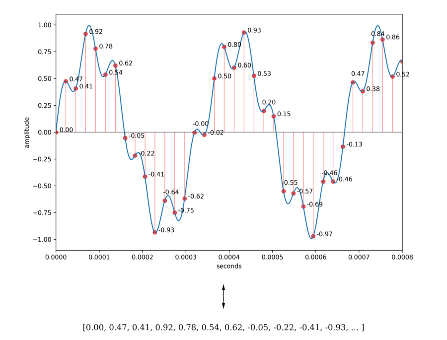
Even though the sampling loses information about the wave; from the sampled data, your computer’s digital-to-analog converter can perfectly reconstruct the portion of the sound that contains all the frequencies up to half of the sampling frequency. This is the Nyquist Theorem. So, assuming our samples are completely accurate, we are O.K. if we choose the sampling frequency to be more than double the maximum frequency humans can hear. Since 22050 is above the human hearing limit, 44100 times per second is a good choice, and, assuming the samples have high precision, we cannot hear the loss of information caused by (non-compressed) digital audio sampled at 44100Hz.
To save time and effort, the loops were down-sampled to 8820Hz. So the bottom four tracks (labeled 8820) contain only 1/5 of the data of the full-resolution tracks; this lower sample rate means the frequencies are limited to 0Hz-4410Hz). Just listening to both versions of each track, it is interesting that 4/5 of the data serves to make the difference between the two versions.
At 8820 Hz, each audio loop corresponds to 16538 (\(d = 16538\)) samples since each is just below two seconds. And we have \(N = 90,333\) of these. We can store all this data in a \(N \times d\) matrix \(X\), which we store in a numpy array. Each row of \(X\) corresponds to an audio loop.
The Average Loop
We can think of each loop as a point in \(\mathbb{R}^d\), we can compute the average of each coordinate to find the average loop. We apply the averaging function to each column of \(X\):
mean_wave = np.apply_along_axis(np.mean, 0, X) Here are the average audio loops, looped a few times for your enjoyment:
These are the normalized versions of the average wave. The actual average is very quiet – likely due to phase cancellation.
The picture over the title is the average of a data-set of pictures of faces. Applying PCA to that data-set gives the ‘eigenfaces’.
What is Principal Component Analysis (PCA)?
Say we, as above, have a data-set consisting of points \((x_{i1},...,x_{id}) \in \mathbb{R}^d.\) We again represent it as a matrix \(X\), whose rows are the data-points. If there are \(N\) data-points, and each point is a vector in \(\mathbb{R}^d\), then \(X\) is an \(N\times d\) matrix.
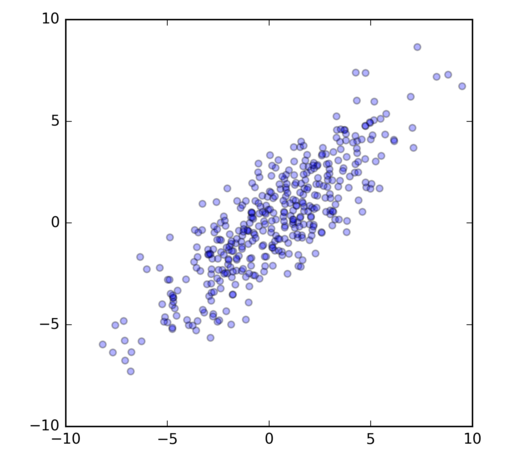
I have a different data-set \(X\) here with \(d = 2\), and \(N = 500\); so \(X\) is a \(500 \times 2\) matrix. If we plotted each point in the data-set (in \(\mathbb{R}^2\)), then it could look like:
Principal Component Analysis (PCA) will find for me the red vectors.
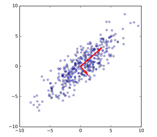
The first (longer) red vector is the first principal component, which is the one direction (in d dimensions) that most accounts for the variation in the point cloud. If I was not allowed to keep 2 numbers for each point in the data, but instead I could only keep one number, the best thing I could do would be to keep the length of the projection onto the first red vector. The second red vector is the remaining orthogonal direction, but in general for \(d>2\), it would be the best among those directions orthogonal to the first vector and so on.
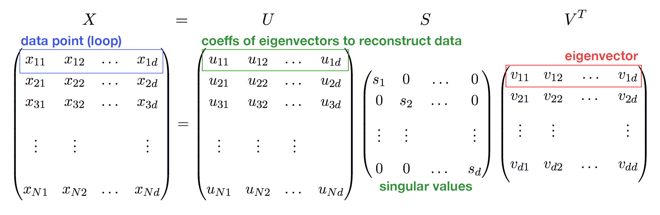
These principal components are obtained using linear algebra, from the Singular Value Decomposition (SVD) of \(X\), which is a process that factorizes \(X\) as a product of three matrices:
\[X = U S V^T\]The red vectors, i.e. principal components, are the rows of \(V^T\), and therefore the columns of \(V\); except that the rows of \(V^T\) all have length \(1\). A matrix like \(V\) whose columns are unit length and orthogonal to each other is called an orthogonal matrix. \(S\) is a diagonal matrix, and the entries in the diagonal are sorted from high to low. These ‘singular values’ represent the length of the red vectors, and describe the amount of variance in the data in the directions of those vectors.
The rows of \(V^T\) are actually the eigenvectors of the matrix \(X^T X\) (a \(d \times d\) matrix; the covariance matrix). That is why people call them eigenvectors. The values in \(S\) are the square roots of the eigenvalues of \(X^T X\).
Applying PCA to the Data
We have to start by removing the mean from the data points to center their mean at the origin. Otherwise, the first principal component will point towards the mean of the data instead of the most significant direction.
X = X - mean_waveWe now apply the Singular Value Decomposition
U, s, Vt = scipy.linalg.svd(X, full_matrices=False)Here is the first eigenvector:
It’s not 100% clean, but it is definitely a bass drum.
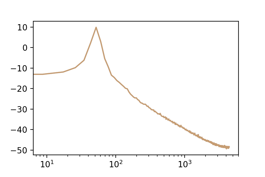
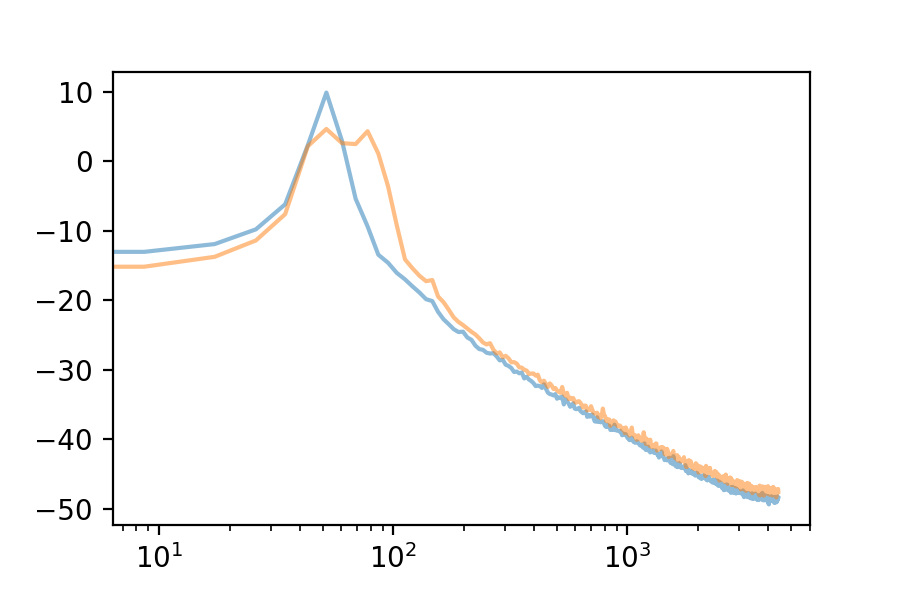
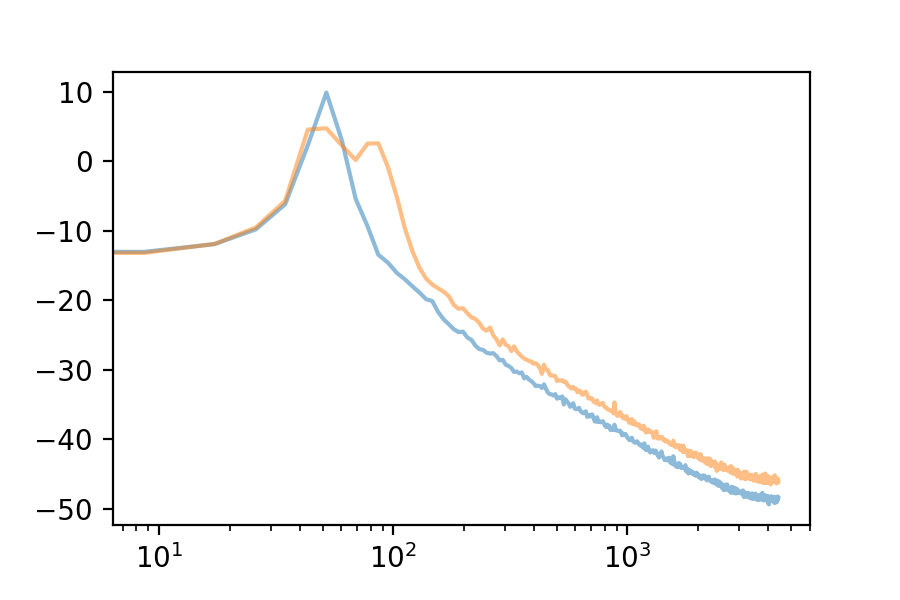
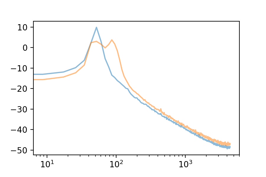
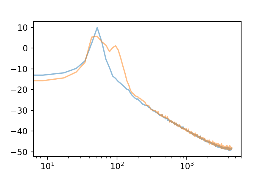
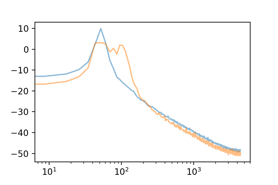
We can use the Fourier Transform to see the frequency spectrum of any loop. The Fourier Transform’s output is an array of complex numbers, containing magnitude and phase information for each frequency bin. Here is the frequency spectrum of the first eigenvector:
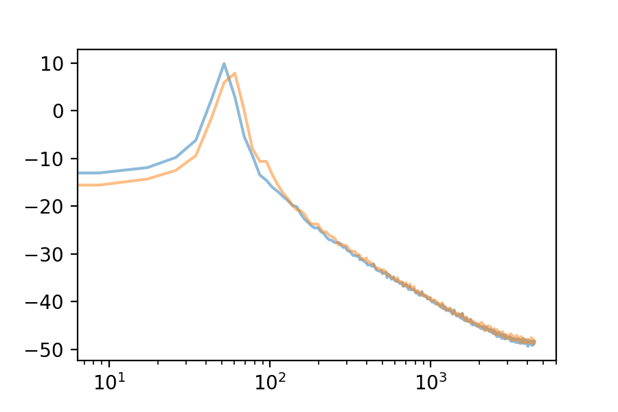
Here are the first 10 eigenvectors. For comparison, I included the first eigenvector’s spectrum in each plot.
| 1 |
</audio> |
| 2 |
 </audio>
 |
| 3 |
 </audio>
 |
| 4 |
 </audio>
 |
| 5 |
 </audio>
 |
| 6 |
 </audio>
 |
| 7 |
 </audio>
 |
| 8 |
 </audio>
 |
| 9 |
 </audio>
 |
| 10 |
 </audio>
 |
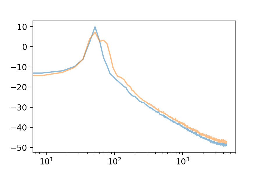
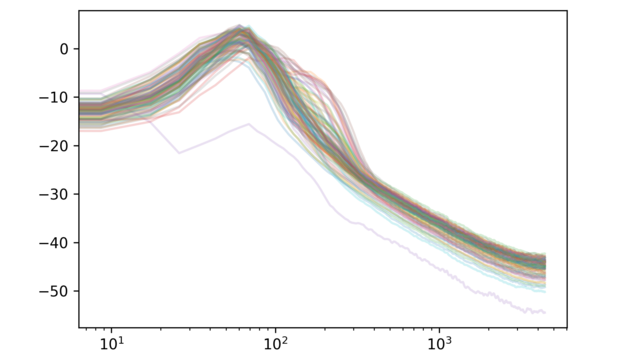
Let’s also look at the spectrum of the first 100 eigenvectors
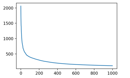
Another tidbit is that the singular values decrease quite sharply:
Approximating Each Loop with the Eigenvectors
How do we write down each loop as as a linear combination of eigenvectors? This what the matrix \(U\) is for. Let
\[\vec{v_1}, \vec{v_2}, \dots , \vec{v_d}\]be all the eigenvectors. Looking at the matrix factorization above, we can write down how we obtain the \(i\)th row on the left, i.e. the \(i\)th loop, from the product on the right:
\[(x_{ij},\dots, x_{id}) = u_{i1}s_1 . \vec{v_1} + u_{i2}s_2 . \vec{v_2} + \dots + u_{id}s_d . \vec{v_d}\]Great, so \(u_{i1}s_1,\dots , u_{id}s_d\) are the coefficients of the eigenvectors that help us make the \(i\)th data vector.
W = U.dot(np.diag(s))Now we can approximate the ith data point by using only the first k eigenvectors in the sum above by:
approxes[i] = W[i,:k].dot(Vt[:k,:])We can do a nice transition going from 0 to all 16538 eigenvectors. So, at the beginning, you will hear just one eigenvector and more and more will be added until we are using all the eigenvectors in the end.
Here are what the specific approximations sound like at various cut-offs:
Here are a few other examples of the same loop approximated with gradually more eigenvectors:
I should note that only the first two examples above are strictly ‘techno’.
Too Much Bass?
The first 10 eigenvectors are very bass-heavy. The same is true for the first 100 eigenvectors. For example the 100th eigenvector sounds like:
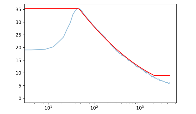
Why does PCA have such a preference for deep bass? Let us look at the average frequency spectrum in our data-set.
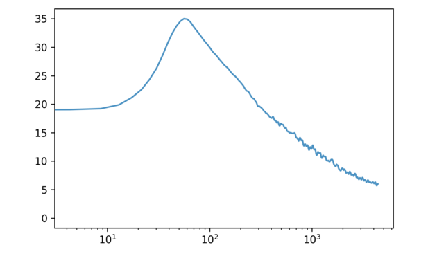
Lower frequencies have higher amplitude. Since SVD is trying to minimize the distance between our data-points and each of their lower-dimensional reconstructions, it makes sense that it would prioritize low frequencies.
Let’s see how the results change if we equalize the frequencies in our data-set (to a reasonable extent). To make the equalizaition, let’s approximate the existing averages using a quadratic – this will allow to make the equalization more smoothly:
And divide the magnitude of the Fourier Transform before applying the inverse to equalize the frequencies in our data-set.
def equalized(X, fscale=freq_scale2):
    ftX = scipy.fft(X)
    for i, x in enumerate(ftX):
        ftX[i] = ftX[i] / fscale(i, slen=X.shape[0])
    return scipy.ifft(ftX).astype(np.float16)
The average spectrum now looks like:
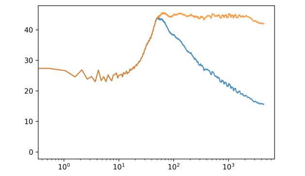
Here is a before/after example of one of the loops:
De-Equalized Results of PCA on the Equalized Data-Set
Running the PCA on the equalized data-set, but then undoing the equalization so that we get approximations of the original data-set, we can think of what we are doing as ‘weighted’ PCA. We are weighting the higher frequencies more to make up for the fact that they appear less in the data-set.
Here are the results of the same analysis on the equalized data-set.
The first 8 eigenvectors are:
These are still kick-drums, but they sound much more like actual kick drums and not just the sub-bass portion of one. Just to compare, this was the first eigenvector before:
Here is eigenvector 20 in the equalized version:
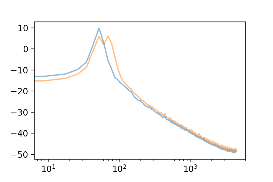
And the spectrum of the first 100 eigenvectors:
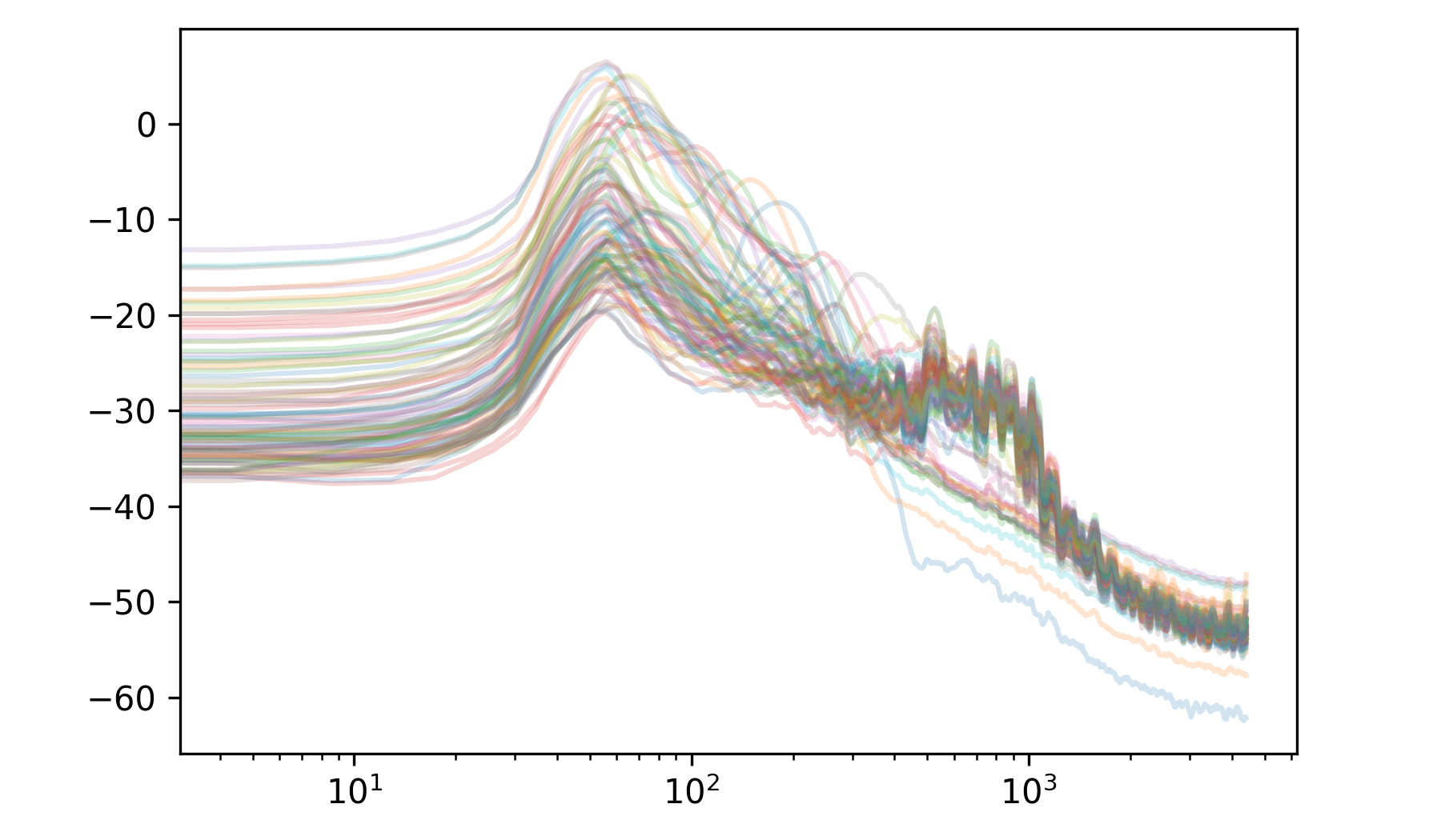
So, as expected, the principal components are branching into the high frequencies much more quickly.
Finally, here are the repeated loops with approximations utilizing more and more of the eigenvectors for the equalized PCA case.
Source code
The dataset
Track credits, in order of appearance:
DJMozart - minimalsound
Hasenchat - Be This Way
Offenbach Project - Vicious Words
Zeropage - Circuit Shaker
Hasenchat - Bulgarian Piccolo
</div>
Hasenchat - Be This Way
Offenbach Project - Vicious Words
Zeropage - Circuit Shaker
Hasenchat - Bulgarian Piccolo </div>