Delay Differentioanl Equations

We follow the lecture notes by Professor Richard Bertram https://www.math.fsu.edu/~bertram/lectures/delay.pdf to present a short introduction to DDE.

A simple example

Recall that for the linear ODE

where $\alpha$ is a given constant, the solution is

Consider positive initial value, i.e., $y(0)>0$. When $\alpha>0$, it is exponentially increasing to infinity as $t\to \infty$ and when $\alpha < 0$, the function decays to zero exponentially.

As a simple example of the delay differential equation (DDE), we change the time variable to $t-1$, i.e.

To solve $\eqref{dde}$, we need function value on $[-1,0]$ more than a single initial value $y(0)$. The dynamic system defined by a delay differential equation is also quite different.

Let's try to solve DDE $\eqref{dde}$. For simplicity, we consider $y = 1$ for $t\in [-1,0]$.

1. For $t\in [0,1]$, the equation can be simplied as $y' = \alpha$ and the solution is

   $$y(t) = \alpha t + 1\quad \text{ for }t\in [0,1].$$

2. With this is known, we can move to the next interval $t\in [1,2]$, the equation becomes

We thus get the quadratic function $y = \frac{1}{2}\alpha^2 t^2 + \alpha t + c$.

3. It is easy to conclude the general solution is:

where the constant $c$ is chosen to glue these pieces continuously.

So this is just the $n$-th Taylor series of $e^{\alpha t}$. For $\alpha>0$, solution $\eqref{ddesolution}$ is also increasing to infinity. But for $\alpha <0$, situation is more complicated. For example, from $\eqref{ddequadratic}$, the minimal point of the quadratic solution is at $-1/\alpha$. Iff $-1/2 < \alpha < 0$, it is out of the interval $[1,2]$ and thus the function is still decreasing. Otherwise, the solution could go up. Namely an oscilation will be observed in the interval $[1,2]$ .

Stability analysis

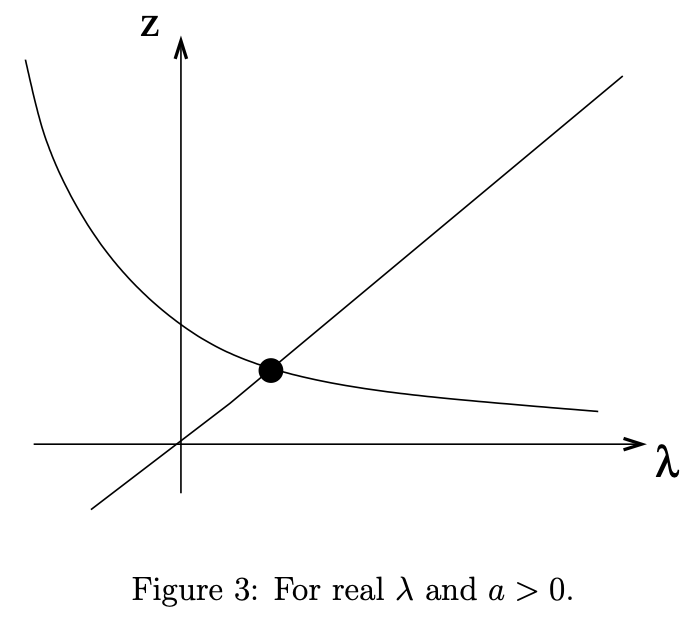
We assume $y = Ce^{\lambda t}$ and substitute into $\eqref{dde}$ to get the so-called characteristic equation of the eigenvalue $\lambda$

This is a transdental equation. When $\alpha>0$, we have one positive real eigenvalue.

When $\alpha <0$, it may have: no solution, one negative real eigenvalue, or two negative real eigenvalues.

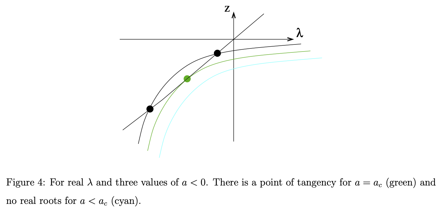
The critical point $\alpha_c = -1/e$. So for the parameter $\alpha_c\leq \alpha <0$, the solution will decay to zero.

How about the case $\alpha < \alpha_c$ ? There is no real eigenvalue. we need to try complex eigenvalues. By introducing the complex eigenvalue $\lambda = \lambda_r + {\rm i} \lambda_i$, the exponential function becomes

Therefore if $\lambda_r<0$, the amplitude $\exp(\lambda_r t)$ will decay to zero and if $\lambda_r>0$ it will increase to infinity. Unlike the real case, since trigonometric functions are involved, oscillation with frequency $\lambda_i$ will be observed. By writing the characterisitc equation in complex numbers, we need to solve

Now there are three unknowns $(\lambda_r, \lambda_i, \alpha)$ but only two equations, so there are infinite solutions to $\eqref{complexeig}$. That is given a parameter $\alpha$, there are infinite many complex eigenvalues.

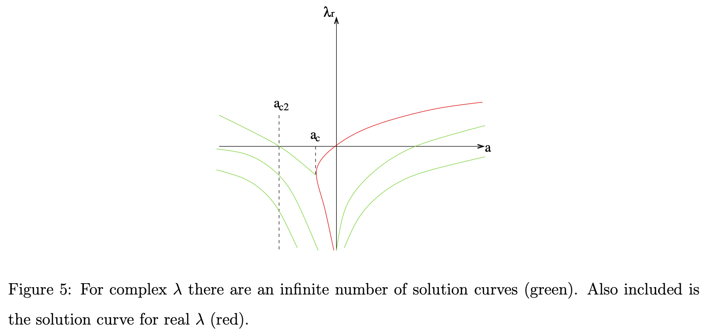
We compute another critical point $\alpha_{c2}$ for which $\lambda_r=0$. By comparing two sides of $\eqref{complexeig}$, we know $\cos \lambda_i =0$, i.e, $\lambda_i = \pm \frac{\pi}{2} + k\pi$ for integer $k$. Then from the imginary part, we conclude

We conclude that for $\alpha \in (-\pi/2, 0)$, the solution will decay to zero but may contain oscillation.

Numerical examples

We include numerical approximation using MATLAB dde23 for several choices of parameter $\alpha$.

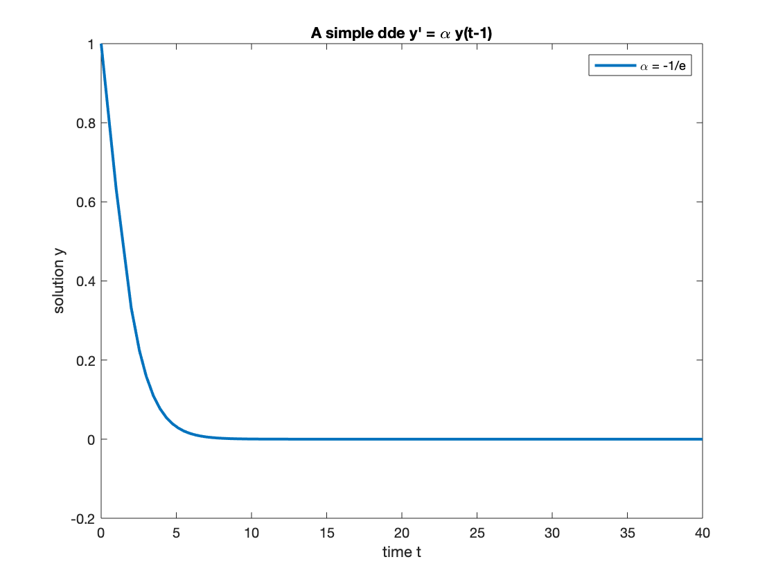
• For real negative eigenvalue, the solution monotonily decrease to zero and behaves like $e^{\alpha t}$. Here we chose the critical point $\alpha_c = -1/e$.
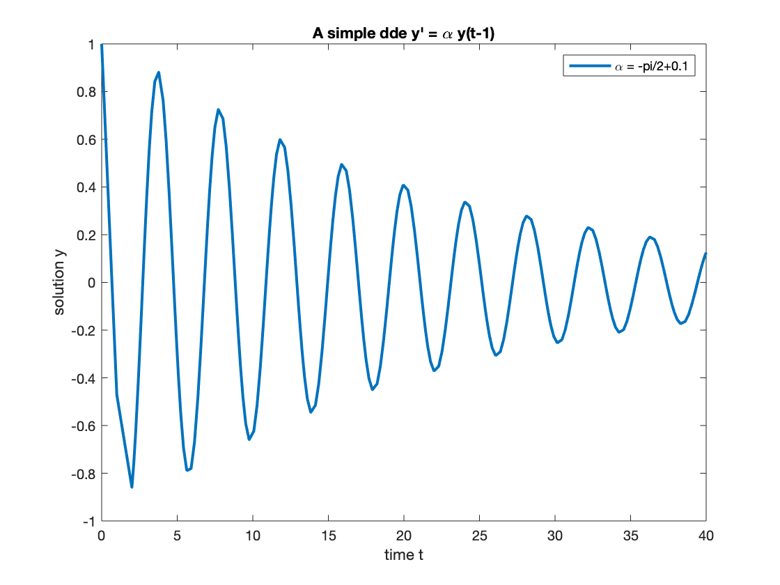
• For complex eigenvalue with negative real part, the solution decays to zero but with oscillations. Here we chose the parameter is slightly less than the critical one $\alpha = -\pi/2 + 0.1$.

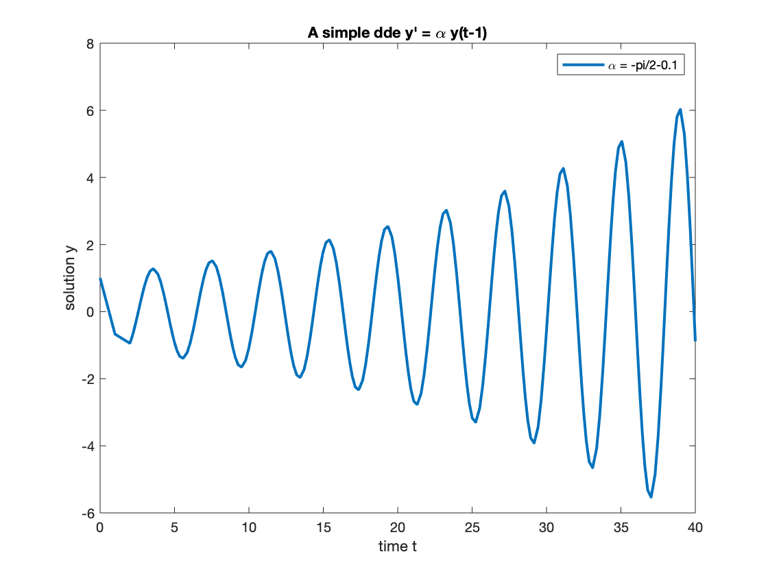
• If we cross the critical point and chose $\alpha = -\pi/2 - 0.1$, then the real part is positive and thus the solution will incresae to infinity but again with oscillations.

  

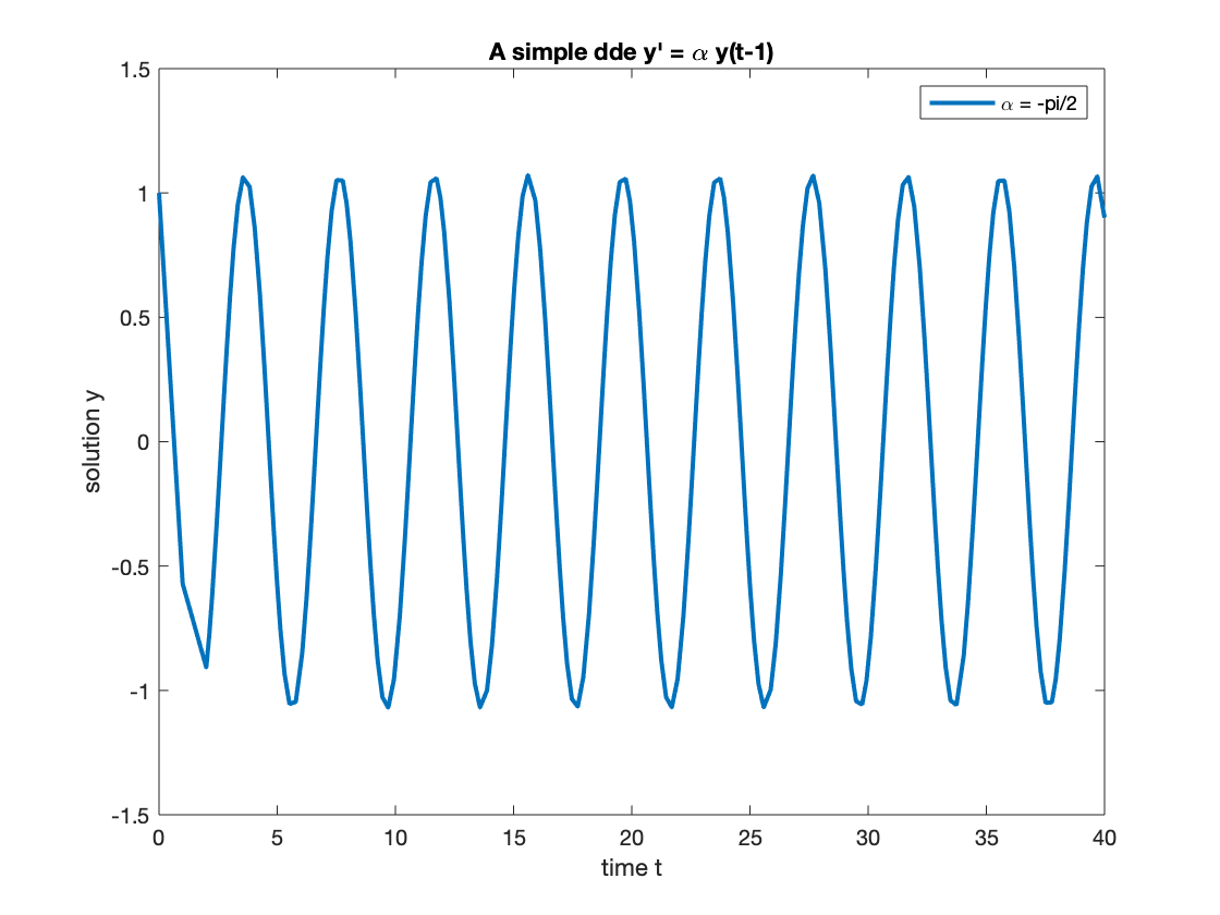
• When $\alpha = -\pi/2$, the ampulity does not change. We get a periodic solution.

Delay Logistic Equation

We first recall the logistic ODE

whose solution is the logist function

The constant $C$ is determined by the initial condition $y(0)$. When $0<y(0) \ll 1$, the function will transit from $y(0)$ to $1$. Recall in the simplest SI model, $I$ behaves like a logistic function and in SIR model, $R$ can be appproximated very well by piecewise logistic functions; see [Perturbation Analysis of SIR model][https://www.math.uci.edu/~chenlong/CAMtips/Coronavirus/SIRperturbation.html].

Now we introduce delay feedback into the logistic equation. Denoted by $y_{\tau} = y(t-1)$ and consider

We are interested in if $y_{\infty} = 1$ is a stable equilibirum of $\eqref{logisticdde}$.

The stability analysis is to assume $y = 1 + \delta y$ with perturbation $|\delta y| \ll 1$. If $\delta y \to 0$ as $t\to \infty$, then $1$ is stable. Otherwise it is unstable.

Substitute into $\eqref{logisticdde}$ and skip the quadratic part, we obtain a simple DDE

for which we have done the stability analysis before. Note that the sign of parameter is changed.

The conclusion is: for $0< \alpha < \pi/2$, $y_{\infty} = 1$ is stable. But for $1/e < \alpha <\pi/2$, it approaches to the steady state will oscillations. We now illustrate by several numerical examples.

• For $\alpha = 1/e \approx 0.3679$, the solution is more or less like the one for standard logistic function. It can be expected that for smaller $0< \alpha < 1/e$, the behavior is similar.

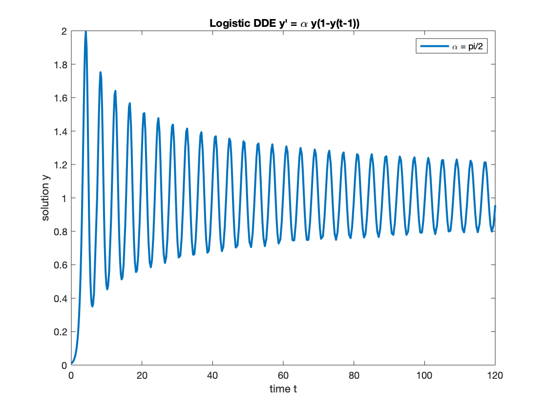
• For $\alpha = \pi/2 - 0.2 \approx 1.3708$, the solution will still approach to $1$ but with oscillation.

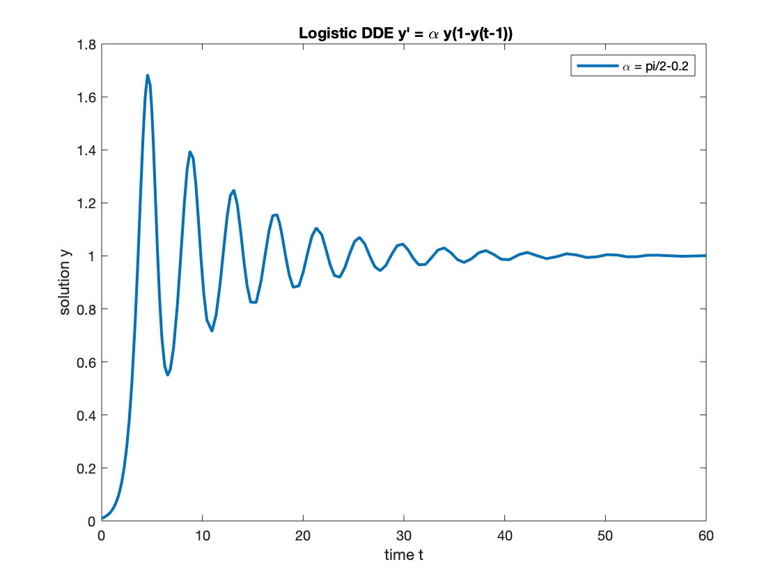
When the solution has some physical or biologic meaning, $y>1$ may not be a meaningful approximation.

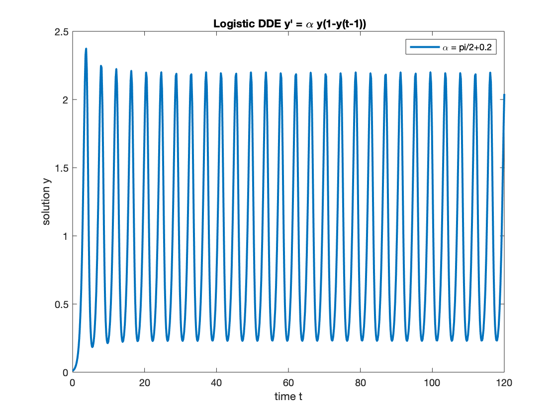
• For $\alpha = \pi/2 + 0.2 \approx 1.7708$, the function doesn't below up but approaches to a periodic function very quickly.

• For $\alpha = \pi/2$, the solution decays to a periodic function with center line $y=1$.