P2 Quadratic Element in 2D
We explain degree of freedoms for quadratic element on triangles. There are two types of dofs: vertex type and edge type. Given a mesh, the required data structure can be constructured by
[elem2dof,edge,bdDof] = dofP2(elem)
Contents
help dofP2
  DOFP2 dof structure for P2 element.

   [elem2dof,edge,bdDof] = DOFP2(elem) constructs the dof structure for the
   quadratic element based on a triangle. elem2dof(t,i) is the global index
   of the i-th dof of the t-th element. Each triangle contains 6 dofs which
   are organized according to the order of nodes and edges, i.e.
   elem2dof(t,1:3) is the pointer to dof on nodes and elem2dof(t,4:6) to
   three edges. The i-th edge is opposited to the i-th vertex.

   See also dof3P2.

   Documentation: <a href="matlab:ifem dofP2doc">P2 Quadratic Element in 2D</a>

  Copyright (C) Long Chen. See COPYRIGHT.txt for details.
Local indexing of DOFs
node = [1,0; 1,1; 0,0];
elem = [1 2 3];
edge = [2 3; 1 3; 1 2];
% elem2dof = 1:6;
figure;
set(gcf,'Units','normal');
set(gcf,'Position',[0,0,0.5,0.3]);
subplot(1,2,1)
showmesh(node,elem);
findnode(node);
findedgedof(node,edge);
subplot(1,2,2)
showmesh(node,elem);
findnode(node);
findedge(node,edge);
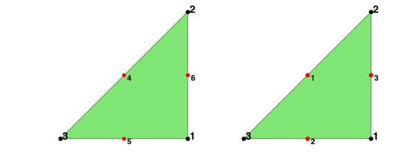
The six dofs in a triangle is displayed in the left. The first three are associated to the vertices of the triangle and the second three to the middle points of three edges. The edges are indexed such that the i-th edge is opposite to the i-th vertex for i=1,2,3.
Local bases of P2
The six Lagrange-type bases functions are denoted by  , i.e.
 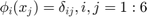 . In barycentric coordinates, they are


When transfer to the reference triangle formed by  , the local bases in x-y coordinate can be obtained by substituting

Global indexing of DOFs
node = [0,0; 1,0; 1,1; 0,1];
elem = [2,3,1; 4,1,3];
[node,elem] = uniformbisect(node,elem);
figure;
showmesh(node,elem);
findnode(node);
findelem(node,elem,'all','index','FaceColor',[0.5 0.9 0.45]);
[elem2dof,edge,bdDof] = dofP2(elem);
findedgedof(node,edge);
The matrix elem2dof is the local to global index mapping of dofs. The first 3 columns, elem2dof(:,1:3), is the global indices of dofs associated to vertexes and thus elem2dof(:,1:3) = elem. The columns elem2dof(:,4:6) point to indices of dofs on edges. The matrix bdDof contains all dofs on the boundary of the mesh.
display(elem2dof);
display(bdDof);
elem2dof =

           8           6           2          14          15          24
           7           6           4          19          20          23
           5           6           1          11          10          22
           9           6           3          16          18          25
           8           3           6          16          24          17
           7           1           6          11          23          12
           5           2           6          14          22          13
           9           4           6          19          25          21


bdDof =

     1
     2
     3
     4
     5
     7
     8
     9
    10
    12
    13
    15
    17
    18
    20
    21