Tutorial of iFEM
Contents
Features of iFEM
- Simple data structures
- Mesh adaptation in two- and three-dimensions
- Fast solvers of algebraic equations
- Easy to use, Easy to code, Easy to debug
- Efficient programming
Basic Data Stucture
Mesh: node and elem.
Two matrices node(1:N,1:d) and elem(1:NT,1:d+1) are used to represent a d-dimensional triangulation embedded in  , where N is the number of vertices and NT is the number of elements.
node(k,1) and node(k,2) are the x- and y-coordinates of the k-th node for points in 2-D. In 3-D, node(k,3) gives the additional z-coordinates of the k-th node.
elem(t,1:d+1) are the global indices of d+1 vertices which form the abstract  -simplex t. By convention, the vertices of a simplex is ordered such that the signed volume is positive. Therefore in 2-D, three vertices of a triangle is ordered counterclockwise and in 3-D, the ordering of vertices follows the right-hand rule.
Related functions: fixorientation, label, label3
Documentation: meshdoc
clear all; close all;
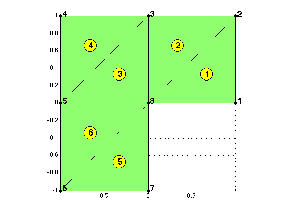
Example: L-shape domain in 2-D.
node = [1,0; 1,1; 0,1; -1,1; -1,0; -1,-1; 0,-1; 0,0];
elem = [1,2,8; 3,8,2; 8,3,5; 4,5,3; 7,8,6; 5,6,8];
figure(1)
showmesh(node,elem)
axis on
findnode(node)
findelem(node,elem)
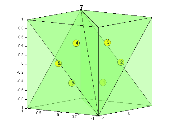
Example: Cube in 3-D.
node = [-1,-1,-1; 1,-1,-1; 1,1,-1; -1,1,-1; -1,-1,1; 1,-1,1; 1,1,1; -1,1,1];
elem = [1,2,3,7; 1,6,2,7; 1,5,6,7; 1,8,5,7; 1,4,8,7; 1,3,4,7];
figure(2)
showmesh3(node,elem,[],'FaceAlpha',0.25);
view([-53,8]);
axis on
findnode3(node)
findelem3(node,elem)
Boundary: bdEdge or bdFace.
For 2-D triangulations, we use bdEdge(1:NT,1:3) to record the type of three edges of each element. Similarly in 3-D, we use bdFace(1:NT,1:4) to record the type of four faces of each element. The value is the type of boundary condition listed as follows.
- 0: non-boundary, i.e., an interior edge or face.
- 1: first type, i.e., a Dirichlet boundary edge or face.
- 2: second type, i.e., a Neumann boundary edge or face.
- 3: third type, i.e., a Robin boundary edge or face.
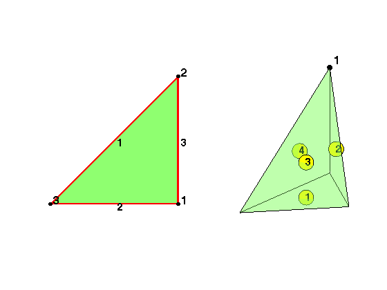
We label three edges of a triangle such that bdEdge(t,i) is the edge opposite to the i-th vertex. Similarly bdFace(t,i) is the face opposite to the i-th vertex.
Related functions: findboundary, setboundary, findboundary3 setboundary3.
Documentation: bddoc
node = [1,0; 1,1; 0,0];
elem = [1 2 3];
edge = [2 3; 1 3; 1 2];
subplot(1,2,1);
showmesh(node,elem);
findedge(node,edge);
findnode(node);
node = [1,1,1; 0,0,0; 1,1,0; 1,0,0];
elem = [1,2,3,4];
subplot(1,2,2);
showmesh3(node,elem,[],'FaceAlpha',0.35); view([-10,18]);
findnode3(node);
findelem3(node,[2,3,4; 1,3,4; 1,2,4; 1,2,3])
Finite Element Method
- Example 1: The Poisson equation in 2-D
- Example 2: The Poisson equation: complex domains
- Example 2: The Poisson equation in 3-D with multigrid solvers
Adaptive Finite Element Method
- Example 1: The Poisson equation on a 2-D L-shaped domain
- Example 2: The Poisson equation in 3-D with jump diffusion coefficients
Time-dependent Problems
- Example 1: Heat equation
- Example 2: Moving interface