Kellogg

KEOLLOGG Problem
Problem setting
Parameters
Generate an initial mesh
Set up PDE data
Adaptive Finite Element Method
Plot convergent rates in energy norm

KEOLLOGG Problem

KELLOGG solves a diffusion equation with jump coefficients with AFEM.

KELLOGG solves the problem within maxN number of vertices. The input argument theta is a parameter used in the marking step.

The KELLOGG command, if no input arguments, use maxN = 5e3 and theta = 0.5.

EXAMPLE

  Kellogg

Problem setting

$-\nabla\cdot(d\nabla u) = 0 \quad \Omega = (-1,1)\times (-1,1)$

$u = g_D \quad \partial \Omega$

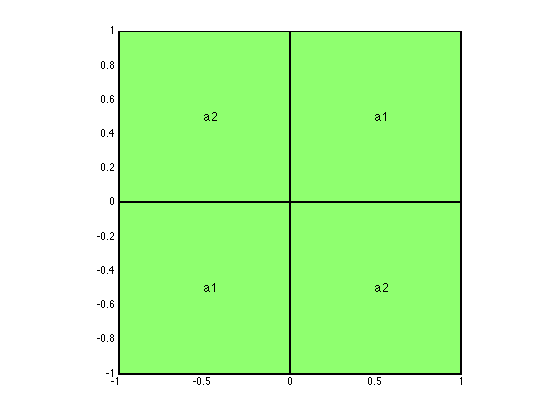
The diffusion constant is discontinous; see the figure below. We set a2 = 1; a1 = 161.4476387975881 and choose boundary condition g_D such that the exact solution is $z = r^{0.1}\mu(\theta)$ in the poloar coordinate, where the formula of mu can be found in exactu function.

[x,y] = meshgrid(-1:1:1,-1:1:1);
z = 0*x;
surf(x,y,z,'linewidth',2); view(2);
axis equal; axis tight;
text(0.5,0.5,'a1','FontSize',12,'FontWeight','bold');
text(-0.5,-0.5,'a1','FontSize',12,'FontWeight','bold');
text(-0.5,0.5,'a2','FontSize',12,'FontWeight','bold');
text(0.5,-0.5,'a2','FontSize',12,'FontWeight','bold');

Parameters

maxN = 3e3;     theta = 0.2;    maxIt = 1000;
N = zeros(maxIt,1);     uIuhErr = zeros(maxIt,1);
errH1 = zeros(maxIt,1);

Generate an initial mesh

[node,elem] = squaremesh([-1 1 -1 1], 0.25);
bdFlag = setboundary(node,elem,'Dirichlet');

Set up PDE data

pde = Kelloggdata;

Adaptive Finite Element Method

SOLVE -> ESTIMATE -> MARK -> REFINE

for k = 1:maxIt
    % Step 1: SOLVE
    [u,Du,eqn] = Poisson(node,elem,pde);
    % Plot mesh and solution
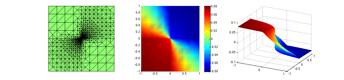
    figure(1);  showresult(node,elem,u,[27,26]);
    % Step 2: ESTIMATE
%    eta = estimaterecovery(node,elem,u);            % recovery type
    eta = estimateresidual(node,elem,u,pde);    % residual type
    % Record error and number of vertices
    uI = pde.exactu(node);
    uIuhErr(k) = sqrt((uI-u)'*eqn.A*(uI-u));
    errH1(k) = getH1error(node,elem,@pde.Du,Du);
    N(k) = size(node,1);
    if (N(k)>maxN), break; end
    % Step 3: MARK
    markedElem = mark(elem,eta,theta);
    % Step 4: REFINE
    [node,elem,bdFlag] = bisect(node,elem,markedElem,bdFlag);
end

Multigrid V-cycle Preconditioner with Conjugate Gradient Method
#dof:     2132,  #nnz:    12344, iter:  8,   err = 5.8395e-09,   time = 0.18 s
Multigrid V-cycle Preconditioner with Conjugate Gradient Method
#dof:     2242,  #nnz:    12986, iter:  8,   err = 3.1593e-09,   time = 0.21 s
Multigrid V-cycle Preconditioner with Conjugate Gradient Method
#dof:     2412,  #nnz:    13940, iter:  8,   err = 3.3831e-09,   time = 0.18 s
Multigrid V-cycle Preconditioner with Conjugate Gradient Method
#dof:     2535,  #nnz:    14631, iter:  8,   err = 4.2176e-09,   time = 0.17 s
Multigrid V-cycle Preconditioner with Conjugate Gradient Method
#dof:     2730,  #nnz:    15708, iter:  8,   err = 6.8518e-09,   time = 0.19 s
Multigrid V-cycle Preconditioner with Conjugate Gradient Method
#dof:     2880,  #nnz:    16522, iter:  8,   err = 6.7943e-09,   time = 0.19 s
Multigrid V-cycle Preconditioner with Conjugate Gradient Method
#dof:     3102,  #nnz:    17692, iter:  8,   err = 6.1075e-09,   time = 0.22 s

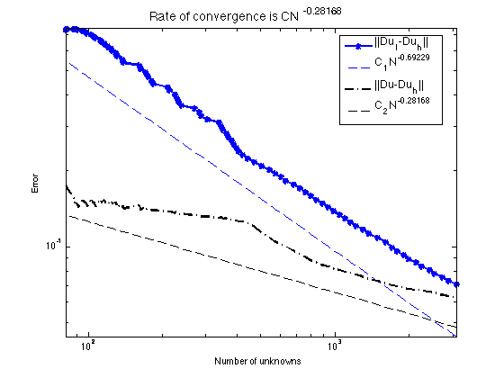
Plot convergent rates in energy norm

N = N(1:k);
uIuhErr = uIuhErr(1:k);
errH1 = errH1(1:k);
figure(2)
showrate2(N,uIuhErr,10,'-*','||Du_I-Du_h||',...
          N,errH1,10,'k-.','||Du-Du_h||');