PoissonQ1femrate

RATE OF CONVERGENCE OF BILINEAR FINITE ELEMENT METHOD
Setting
Non-empty Dirichlet boundary condition.
Pure Neumann boundary condition.
Pure Robin boundary condition.
Conclusion

RATE OF CONVERGENCE OF BILINEAR FINITE ELEMENT METHOD

This example is to show the rate of convergence of bilinear finite element approximation of the Poisson equation on the unit square:

$- \Delta u = f \; \hbox{in } (0,1)^2$

for the following boundary condition:

Non-empty Dirichlet boundary condition. $u=g_D \hbox{ on }\Gamma_D, \quad \nabla u\cdot n=g_N \hbox{ on }\Gamma_N. \Gamma _D = \{(x,y): x=0, y\in [0,1]\}, \; \Gamma _N = \partial \Omega \backslash \Gamma _D$ .
Pure Neumann boundary condition. $\Gamma _N = \partial \Omega$ .
Robin boundary condition. $g_R u + \nabla u\cdot n=g_N \hbox{ on }\partial \Omega$

clear variable

Setting

[node,elem] = squarequadmesh([0,1,0,1],1/2^3);
mesh  = struct('node',node,'elem',elem);
option.L0 = 2;
option.maxIt = 4;
option.printlevel = 1;
option.plotflag = 0;
option.elemType = 'Q1';

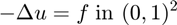
Non-empty Dirichlet boundary condition.

pde = sincosdata;
mesh.bdFlag = setboundary(node,elem,'Dirichlet','~(x==0)','Neumann','x==0');
femPoisson(mesh,pde,option);

Multigrid V-cycle Preconditioner with Conjugate Gradient Method
#dof:     4225,  #nnz:    35530, smoothing: (1,1), iter:  7,   err = 3.84e-09,   time = 0.017 s
Multigrid V-cycle Preconditioner with Conjugate Gradient Method
#dof:    16641,  #nnz:   144778, smoothing: (1,1), iter:  7,   err = 6.20e-09,   time = 0.063 s
Multigrid V-cycle Preconditioner with Conjugate Gradient Method
#dof:    66049,  #nnz:   584458, smoothing: (1,1), iter:  7,   err = 9.62e-09,   time = 0.21 s

 #Dof       h       ||u-u_h||    ||Du-Du_h||   ||DuI-Du_h|| ||uI-u_h||_{max}

 1089   3.12e-02   7.57200e-04   4.44017e+00   8.53343e-04   2.71970e-04
 4225   1.56e-02   1.89319e-04   4.44220e+00   2.13806e-04   6.79552e-05
16641   7.81e-03   4.73308e-05   4.44271e+00   5.34807e-05   1.69906e-05
66049   3.91e-03   1.18328e-05   4.44284e+00   1.33715e-05   4.24808e-06

 #Dof   Assemble     Solve      Error      Mesh    

 1089   1.00e-02   1.92e-03   2.00e-02   1.00e-02
 4225   7.00e-02   1.67e-02   1.00e-01   1.00e-02
16641   2.20e-01   6.32e-02   2.90e-01   5.00e-02
66049   8.10e-01   2.14e-01   9.20e-01   2.00e-01

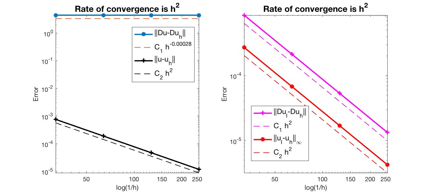
Pure Neumann boundary condition.

pde = sincosNeumanndata;
mesh.bdFlag = setboundary(node,elem,'Neumann');
femPoisson(mesh,pde,option);

Multigrid V-cycle Preconditioner with Conjugate Gradient Method
#dof:     4225,  #nnz:    37242, smoothing: (1,1), iter:  9,   err = 4.35e-10,   time = 0.017 s
Multigrid V-cycle Preconditioner with Conjugate Gradient Method
#dof:    16641,  #nnz:   148218, smoothing: (1,1), iter:  9,   err = 1.68e-09,   time = 0.051 s
Multigrid V-cycle Preconditioner with Conjugate Gradient Method
#dof:    66049,  #nnz:   591354, smoothing: (1,1), iter:  9,   err = 9.54e-09,   time = 0.25 s

 #Dof       h       ||u-u_h||    ||Du-Du_h||   ||DuI-Du_h|| ||uI-u_h||_{max}

 1089   3.12e-02   1.89964e-03   8.87506e+00   1.42236e-02   3.21831e-03
 4225   1.56e-02   5.39236e-04   8.88372e+00   4.90169e-02   4.88870e-02
16641   7.81e-03   1.34875e-04   8.88525e+00   2.45349e-02   2.45187e-02
66049   3.91e-03   3.37228e-05   8.88564e+00   1.22707e-02   1.22687e-02

 #Dof   Assemble     Solve      Error      Mesh    

 1089   1.00e-02   2.49e-03   1.00e-02   0.00e+00
 4225   6.00e-02   1.68e-02   9.00e-02   1.00e-02
16641   2.30e-01   5.15e-02   2.30e-01   5.00e-02
66049   8.20e-01   2.46e-01   1.00e+00   2.00e-01

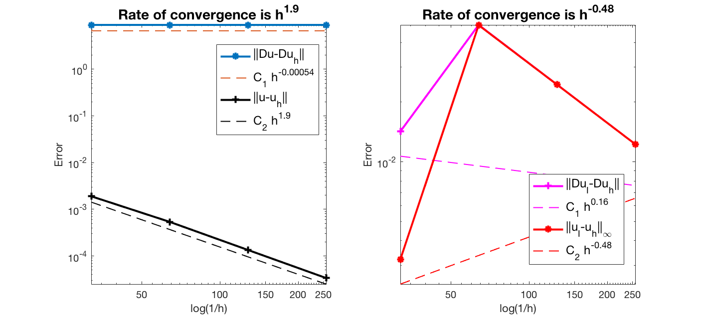
Pure Robin boundary condition.

option.plotflag = 0;
pde = sincosRobindata;
mesh.bdFlag = setboundary(node,elem,'Robin');
femPoisson(mesh,pde,option);

Multigrid V-cycle Preconditioner with Conjugate Gradient Method
#dof:     4225,  #nnz:    37249, smoothing: (1,1), iter:  7,   err = 1.38e-09,   time = 0.018 s
Multigrid V-cycle Preconditioner with Conjugate Gradient Method
#dof:    16641,  #nnz:   148225, smoothing: (1,1), iter:  7,   err = 2.31e-09,   time = 0.056 s
Multigrid V-cycle Preconditioner with Conjugate Gradient Method
#dof:    66049,  #nnz:   591361, smoothing: (1,1), iter:  7,   err = 3.45e-09,   time = 0.24 s

 #Dof       h       ||u-u_h||    ||Du-Du_h||   ||DuI-Du_h|| ||uI-u_h||_{max}

 1089   3.12e-02   1.89975e-03   8.87506e+00   1.45807e-02   3.21823e-03
 4225   1.56e-02   4.75115e-04   8.88309e+00   3.65461e-03   8.03533e-04
16641   7.81e-03   1.18790e-04   8.88510e+00   9.14242e-04   2.00819e-04
66049   3.91e-03   2.96981e-05   8.88560e+00   2.28597e-04   5.02008e-05

 #Dof   Assemble     Solve      Error      Mesh    

 1089   1.00e-02   2.15e-03   1.00e-02   0.00e+00
 4225   7.00e-02   1.75e-02   1.10e-01   1.00e-02
16641   2.20e-01   5.60e-02   2.70e-01   5.00e-02
66049   8.80e-01   2.38e-01   1.04e+00   2.50e-01

Conclusion