RATE OF CONVERGENCE OF LINEAR FINITE ELEMENT METHOD
This example is to show the rate of convergence of linear finite element approximation of the Poisson equation on the unit square:
for the following boundary condition:
- Non-empty Dirichlet boundary condition.
![$u=g_D \hbox{ on }\Gamma_D, \quad \nabla u\cdot n=g_N \hbox{ on }\Gamma_N. \Gamma _D = \{(x,y): x=0, y\in [0,1]\}, \; \Gamma _N = \partial \Omega \backslash \Gamma _D$](femrateP2_eq34764.png) .
. - Pure Neumann boundary condition.
 .
. - Robin boundary condition.

Contents
clear all; close all; clc;
[node,elem] = squaremesh([0,1,0,1],0.25);
option.L0 = 1;
option.maxIt = 4;
option.printlevel = 1;
option.plotflag = 0;
option.elemType = 'P2';
format shorte
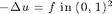
Non-empty Dirichlet boundary condition.
pde = sincosdata;
bdFlag = setboundary(node,elem,'Dirichlet','~(x==0)','Neumann','x==0');
err = femPoisson(node,elem,pde,bdFlag,option);
Multigrid V-cycle Preconditioner with Conjugate Gradient Method
#dof:     4225,  #nnz:    39184, iter: 10,   err = 2.6755e-09,   time = 0.52 s
Multigrid V-cycle Preconditioner with Conjugate Gradient Method
#dof:    16641,  #nnz:   160272, iter: 10,   err = 5.4569e-09,   time = 0.51 s
display('   ||u-u_h||   ||Du-Du_h||  ||DuI-Du_h||  ||uI-u_h||_{max}');
display([err.L2 err.H1 err.uIuhH1 err.uIuhMax]);
   ||u-u_h||   ||Du-Du_h||  ||DuI-Du_h||  ||uI-u_h||_{max}

ans =

   4.5722e-04   2.1682e-02   4.5133e-03   6.7421e-04
   5.7049e-05   5.4875e-03   6.9756e-04   8.8853e-05
   7.1342e-06   1.3779e-03   1.1074e-04   1.1453e-05
   8.9219e-07   3.4505e-04   1.8246e-05   1.4548e-06
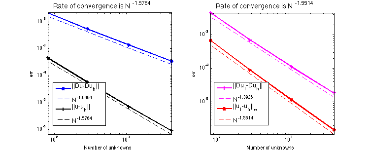
Pure Neumann boundary condition.
pde = sincosNeumanndata;
bdFlag = setboundary(node,elem,'Neumann');
err = femPoisson(node,elem,pde,bdFlag,option);
Multigrid V-cycle Preconditioner with Conjugate Gradient Method
#dof:     4225,  #nnz:    41458, iter: 10,   err = 5.8429e-09,   time = 0.53 s
Multigrid V-cycle Preconditioner with Conjugate Gradient Method
#dof:    16641,  #nnz:   164850, iter: 11,   err = 3.9313e-09,   time =  1.3 s
display('   ||u-u_h||   ||Du-Du_h||  ||DuI-Du_h||  ||uI-u_h||_{max}');
display([err.L2 err.H1 err.uIuhH1 err.uIuhMax]);
   ||u-u_h||   ||Du-Du_h||  ||DuI-Du_h||  ||uI-u_h||_{max}

ans =

   1.3592e-02   1.5713e-01   8.9370e-02   2.6274e-02
   2.0398e-03   4.2201e-02   1.5150e-02   3.9808e-03
   2.7330e-04   1.0834e-02   2.5578e-03   5.3478e-04
   3.5211e-05   2.7383e-03   4.3864e-04   6.8974e-05
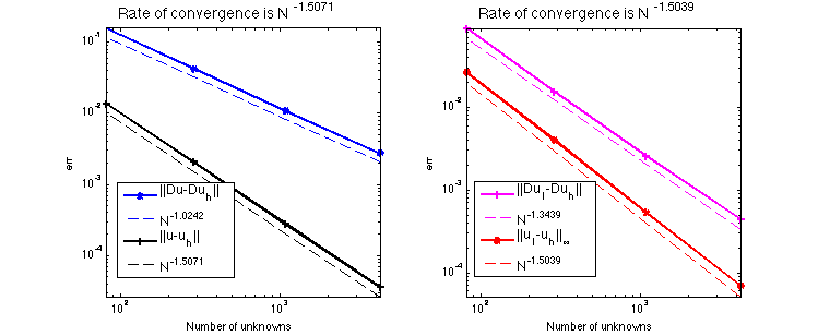
Pure Robin boundary condition.
option.plotflag = 0;
pdeRobin = sincosRobindata;
bdFlag = setboundary(node,elem,'Robin');
err = femPoisson(node,elem,pdeRobin,bdFlag,option);
Multigrid V-cycle Preconditioner with Conjugate Gradient Method
#dof:     4225,  #nnz:    41473, iter:  9,   err = 8.3083e-09,   time =  1.1 s
Multigrid V-cycle Preconditioner with Conjugate Gradient Method
#dof:    16641,  #nnz:   164865, iter: 10,   err = 2.5881e-09,   time = 0.98 s
display('   ||u-u_h||   ||Du-Du_h||  ||DuI-Du_h||  ||uI-u_h||_{max}');
display([err.L2 err.H1 err.uIuhH1 err.uIuhMax]);
   ||u-u_h||   ||Du-Du_h||  ||DuI-Du_h||  ||uI-u_h||_{max}

ans =

   3.4930e-03   1.5715e-01   8.9472e-02   1.2867e-02
   4.4650e-04   4.2204e-02   1.5165e-02   1.9596e-03
   5.6508e-05   1.0834e-02   2.5598e-03   2.6443e-04
   7.1046e-06   2.7384e-03   4.3889e-04   3.4231e-05
Conclusion
The optimal rate of convergence of the H1-norm (2nd order) and L2-norm (3rd order) is observed. The order of |DuI-Duh| is almost 3rd order and thus superconvergence exists.
MGCG converges uniformly in all cases.