Project: 1-D Finite Difference Method

The purpose of this project is to introduce the finite difference. We use 1-D Poisson equation in (0,1) with Dirichlet boundary condition

$- u'' = f \, (0,1), \quad u(0) = a, u(1) = b.$

Step 1: Generate a grid
Step 2: Generate a matrix equation
Stpe 3: Modify the matrix and right hand side to impose boundary condition
Step 4: Test of code
Step 5: Check the Convergence Rate

Step 1: Generate a grid

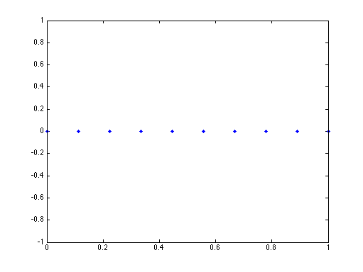
Generate a vector representing a uniform grid with size h of (0,1).

N = 10;
x = linspace(0,1,N);
plot(x,0,'b.','Markersize',16)

Step 2: Generate a matrix equation

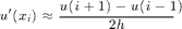
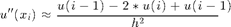
Based on the grid, the function $u$ is discretized by a vector u. The derivative $u', u''$ are approximated by centeral finite difference:

$u'(x_i) \approx \frac{u(i+1) - u(i-1)}{2h}$

$u''(x_i) \approx \frac{u(i-1) - 2*u(i) + u(i-1)}{h^2}$

The equation $-u''(x) = f(x)$ is discretized at $x_i, i=1,...,N$ as

$\frac{-u(i-1) + 2*u(i) - u(i-1)}{h^2} \quad = f(i)$

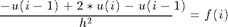
where $f(i) = f(x_i)$ . These linear equations can be written as a matrix equation A*u = f, where A is a tri-diagonal matrix (-1,2,-1)/h^2.

n = 5;
e = ones(n,1);
A = spdiags([e -2*e e], -1:1, n, n);
display(full(A));

ans =

    -2     1     0     0     0
     1    -2     1     0     0
     0     1    -2     1     0
     0     0     1    -2     1
     0     0     0     1    -2

We use spdiags to speed up the generation of the matrix. If using diag, ....

Stpe 3: Modify the matrix and right hand side to impose boundary condition

The discretization fails at boundary vertices since no nodes outside the interval. Howevery the boundary value is given by the problem: u(1) = a, u(N) = b.

These two equations can be included in the matrix by changing A(1,:) = [1, 0 ..., 0] and A(:,N) = [0, 0, ..., 1] and |f(1) = a/h^2, f(N) = b/h^2.

A(1,1) = 1;
A(1,2) = 0;
A(n,n) = 1;
A(n,n-1) = 0;
display(full(A));

ans =

     1     0     0     0     0
     1    -2     1     0     0
     0     1    -2     1     0
     0     0     1    -2     1
     0     0     0     0     1

Step 4: Test of code

[u,x] = poisson1D(0,1,5);
plot(x,sin(x),x,u,'r*');
legend('exact solution','approximate solution')

Undefined function 'poisson1D' for input arguments of type 'double'.

Error in projectFDM1D (line 54)
[u,x] = poisson1D(0,1,5);

We test ... The result seems correct since the computed solution fits well on the curve of the true solution.

Step 5: Check the Convergence Rate

err = zeros(4,1);
h = zeros(4,1);
for k = 1:4
    [u,x] = poisson1D(0,1,2^k+1);
    uI = sin(x);
    err(k) = max(abs(u-uI));
    h(k) = 1/2^k;
end
display(err)
loglog(h,err,h,h.^2);
legend('error','h^2');
axis tight;