Project: Edge Finite Element Method for Maxwell-type Equations
The purpose of this project is to implement the lowest order edge element for solving the following Maxwell equations in three dimensions

with Dirichlet boundary condition  on
on 
The vector function  is approximated by the lowest order edge element. To impose the divergence constraint, a Lagrange multiplier
  is introduced and approximated by the linear element. Convergence theory can be found in my lecture notes:
Contents
Step 1: Data Structure
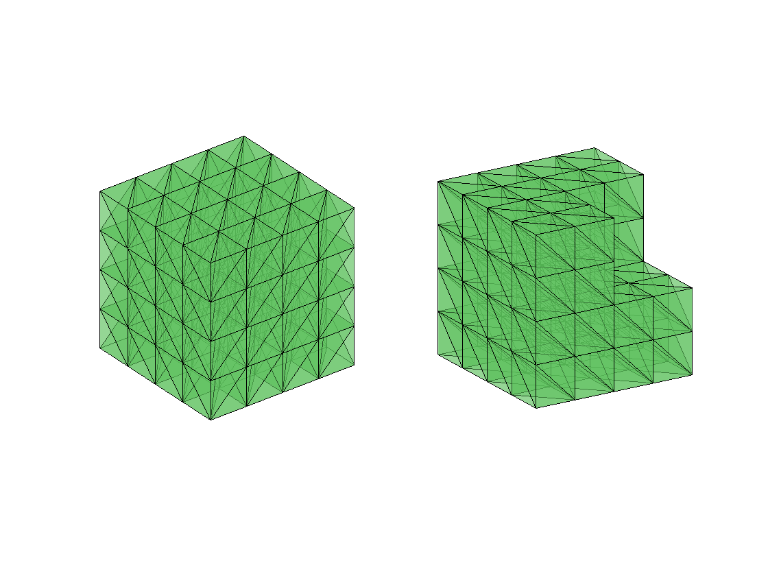
A three dimensional mesh is still represented by node, elem. A mesh for a cube can be obtained
[node,elem] = cubemesh([-1,1,-1,1,-1,1],0.5);
figure(1); subplot(1,2,1); showmesh3(node,elem);

% A mesh for an L-shaped domain
[node,elem] = cubemesh([-1,1,-1,1,-1,1],0.5);
[node,elem] = delmesh(node,elem,'x<0 & y<0 & z>0');
figure(1); subplot(1,2,2); showmesh3(node,elem); view(-122,20);
Since the unknowns are associated to edges, you need to generate edges and more importantly the indices map from one tetrahedron to global indices of its six edges. The orientation of local edges of a tetrahedron formed by [1 2 3 4] is lexicographic order: [1 2], [1 3], [1 4], [2 3], [2 4], [3 4] The global orientation of edge is from the node with smaller index to bigger one. elem2edgeSign records the consistency of the local and global edge orientation.
Doc: href="matlab:ifem dof3edgedoc">dof3edgedoc</a
[elem2edge,edge,elem2edgeSign] = dof3edge(elem);
Step 2: Assemble matrices
Suppose [i,j] is the kth edge and orientated from i to j. The basis associated to the kth edge is given by
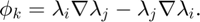
Use the following subroutine to generate 
[Dlambda,volume] = gradbasis3(node,elem);
and compute the piecewise constant vector 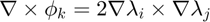 . Then the entry
  can be computed accordingly. When assemble the local entry to the global one, don't forgot the sign consistency.
The computation of (negative) weak divergence of an edge element is changed to compute the inner product  which is a linear combination of the entry
Step 3: Right hand side
Use one point quadrature to compute  Remember to correct the sign.
Step 4: Modify equations to include boundary conditions
Modify the right hand side to include Dirichlet boundary conditions. First of all, to set up the boundary condition use
bdFlag = setboundary3(node,elem,'Dirichlet');
To find out the boundary edges and boundary nodes, use
[bdEdge,bdNode,isBdEdge,isBdNode] = findboundaryedge3(edge,elem2edge,bdFlag);
Boundary nodes since the boundary condition for the Lagrange multiplier is zero on boundary nodes.
The boundary value associated to edges on the boundary is given by the edge integral

Use Simpson rule to compute an approximation of the above integral.
Step 5: Solve the linear system
- Use the direct solver \ to solve the linear system - (optional) Implement DGS Multi-Grid method to solve the system
Step 6: Verify the convergence
- Substitude a smooth function into the equation to get a right hand side. Pass the data f and g_D to your subroutine to compute an approximation u.
- Compute the edge interpolant u_I by computing edge integrals using the exact formula of u.
- Compare u_I and u_h in the energy norm using the curl-curl matrix.
- Compute the error p in the H1 norm.
- Refine mesh several times and show the order of convergences.
[node,elem,bdFlag] = uniformrefine3(node,elem,bdFlag);