Project: Transient Navier-Stokes Equations
The purpose of this project is to implement numerical methods for solving time-dependent Navier-Stokes equations in two dimensions.
Contents
Problem setting: Flow past a cylinder
The domain is

The center of the cylinder is slightly off the center of the channel vertically which eventually leads to asymmetry in the flow.
We are solving the Navier-Stokes equation


The time-dependent inflow boundary condition on the left is

The outflow boundary condition on the right  is
is

On the other part of the boundary, no-slip boundary condition  is imposed.
The initial condition is zero 
The body force is zero too 
We choose  Since the maximum velocity is one and the diameter of the cylinder is 0.1, the Reynolds number of the flow is 100.
Step 1: Mesh
Download the mesh flowpastcylindermesh.mat and load it in Matlab.
load flowpastcylindermesh
showmesh(node,elem); axis on; axis tight;
set(gcf,'Units','normal');
set(gcf,'Position',[0.125,0.125,0.35,0.2]);

When uniform refine this coarse grid, you need to project the circular part back to the circle.
Step 2: FEM for convection-diffusion-reaction equations
Choose either non-conforming P1 - P0 or iso P2-P0 elements.
Besides the matrix for Laplacian and divergence operator, you need to compute one more matrix for the convection term  and the mass matrix for the reaction term
The mass matrix for non-conforming P1 is diagonal. For P1 element, use mass lumping to compute a diagonal mass matrix.
For convection term, first write out component-wise weakformulation and compute the element-wise entry and finally assemble the matrix. Note that the derivative of a linear basis is constant which can be factor out the integral and one-point quadrature is good enough.
Test your code for a scalar convection-diffusion-reaction equation

by choosing a smooth function and moderate convection coefficient.
Step 3: Time Discretization and Nonlinear Iteration for N-S equations
- Implement Crack-Nicolson method for time discretization with dt = 0.0025 which leads in each discrete time step to a non-linear system of equations.
- Use Picard (fixed point) iteration to solve the nonlinear problem. The fixed point iteration was stopped if the Euclidean norm of the residual vector was less than 1e-8.
- Discretization of the linear systems in space by either non-conforming P1 - P0 or isoP2-P0 elements. Solve the algebraic system using direct solver (backslash) in Matlab.
Step 4: GMRES method for solving the linearied problem
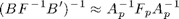
Suppose the linear saddle point system system is [ F B'; B 0 ]. Use the block-triangular preconditioner [F B'; 0 -BF^{-1}B']^{-1} and GMRES to solve the linear system to the tolerence 1e-6.
The inverse of the Schur complement is approximated by the least-square commutator
where

The Poisson solver  can be replaced by the direct solver or one V-cycle.