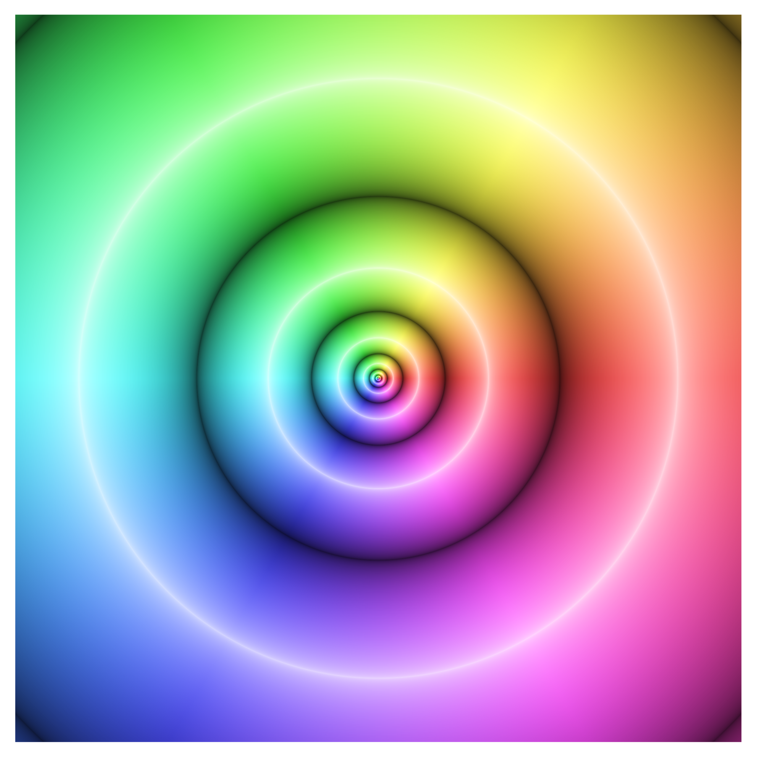
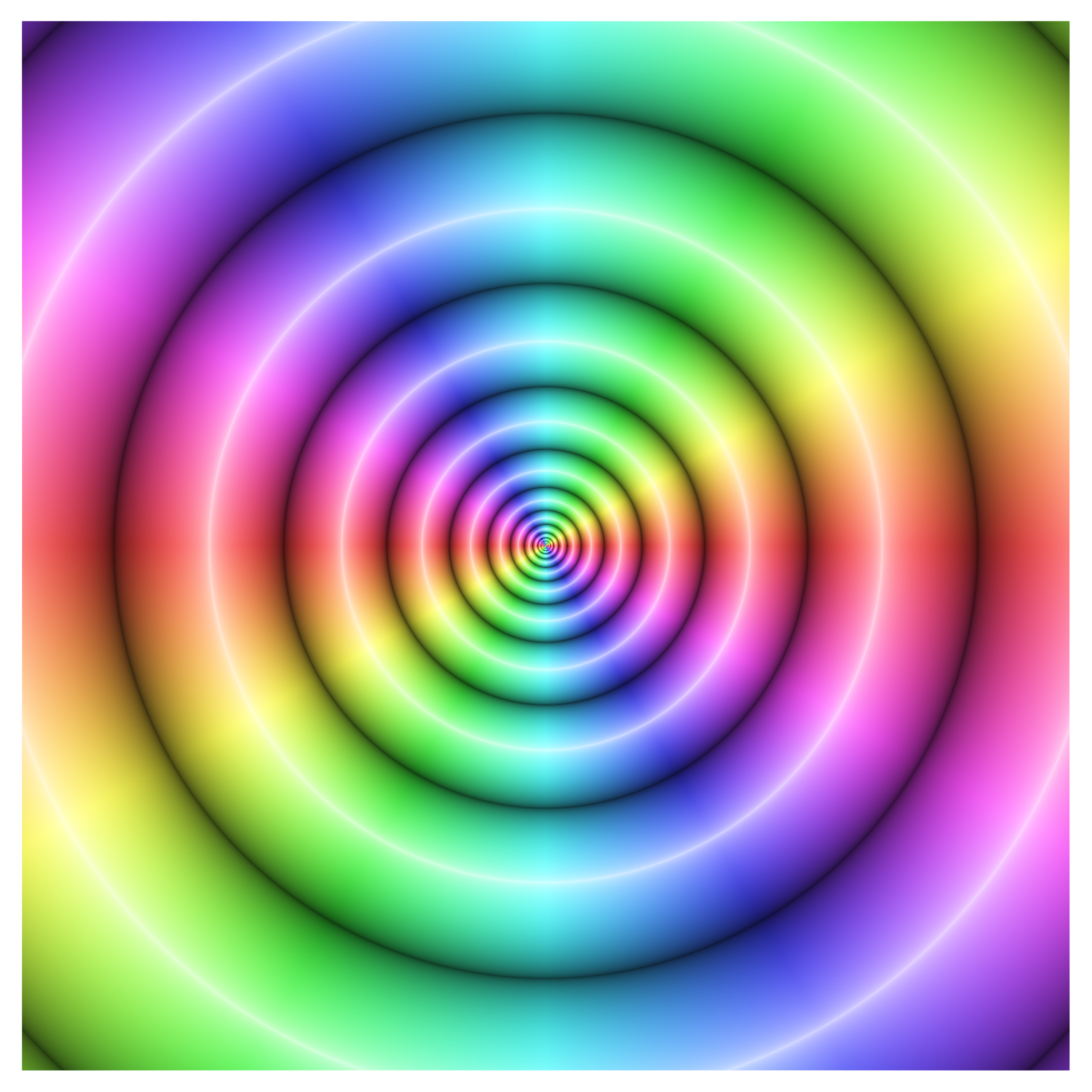
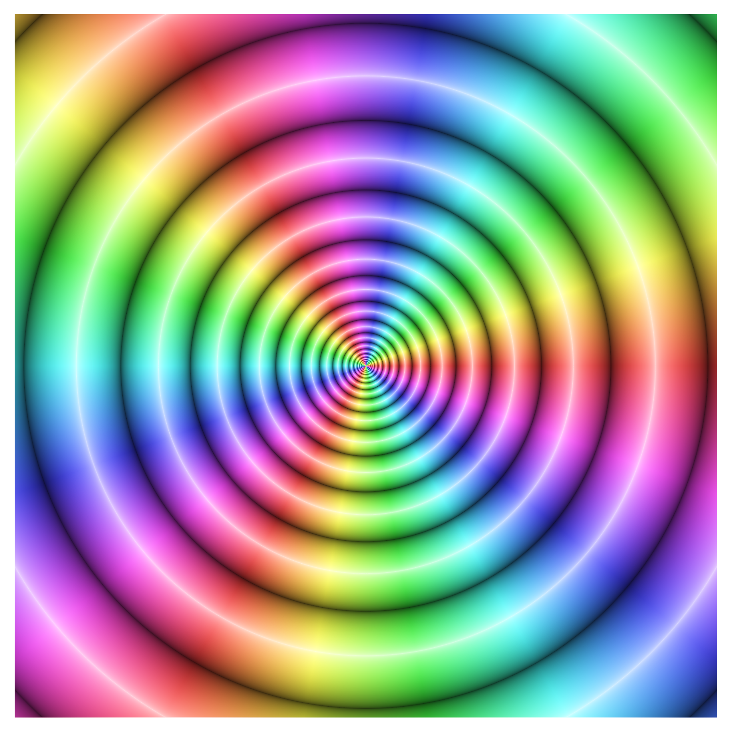
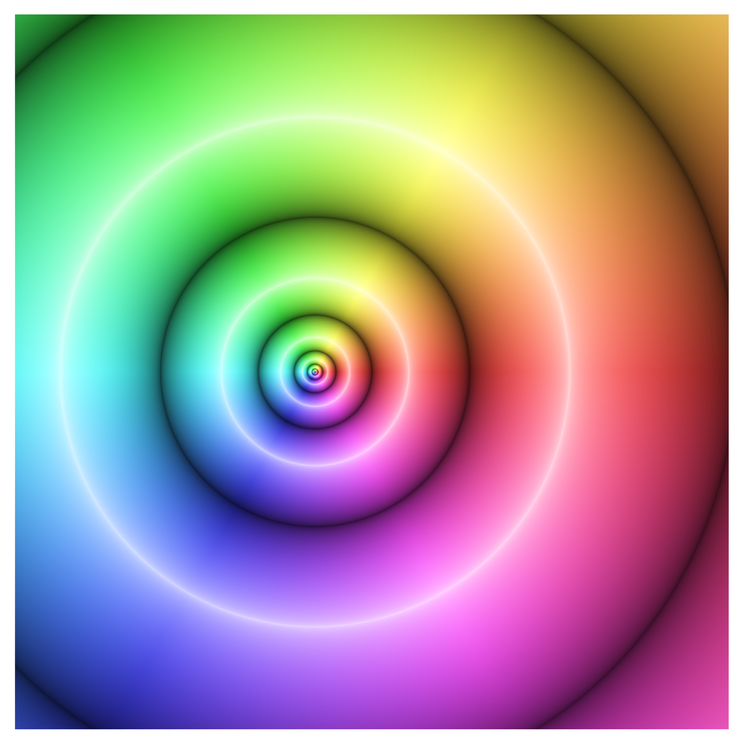
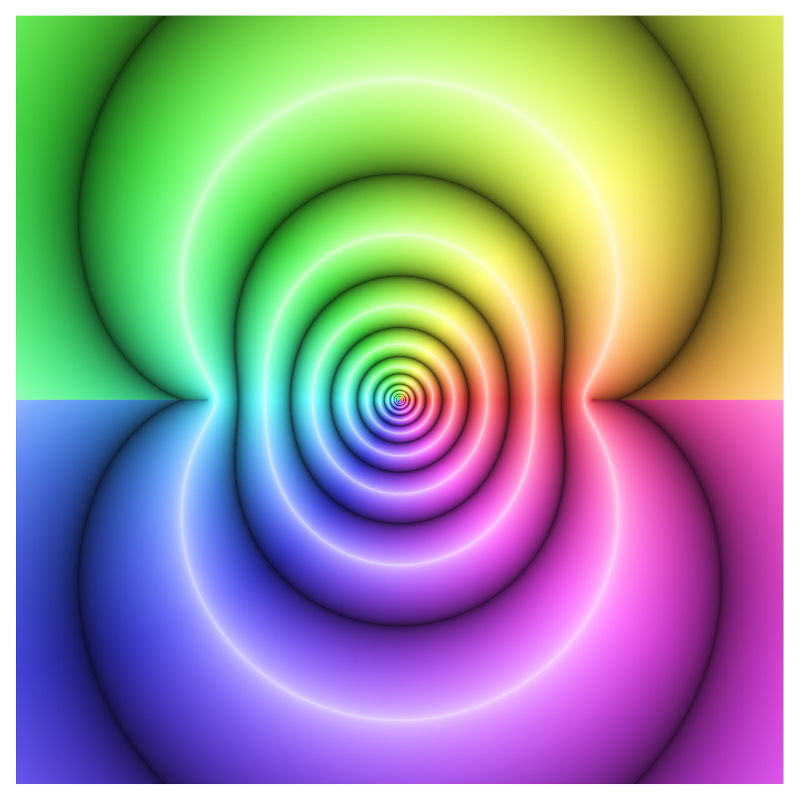
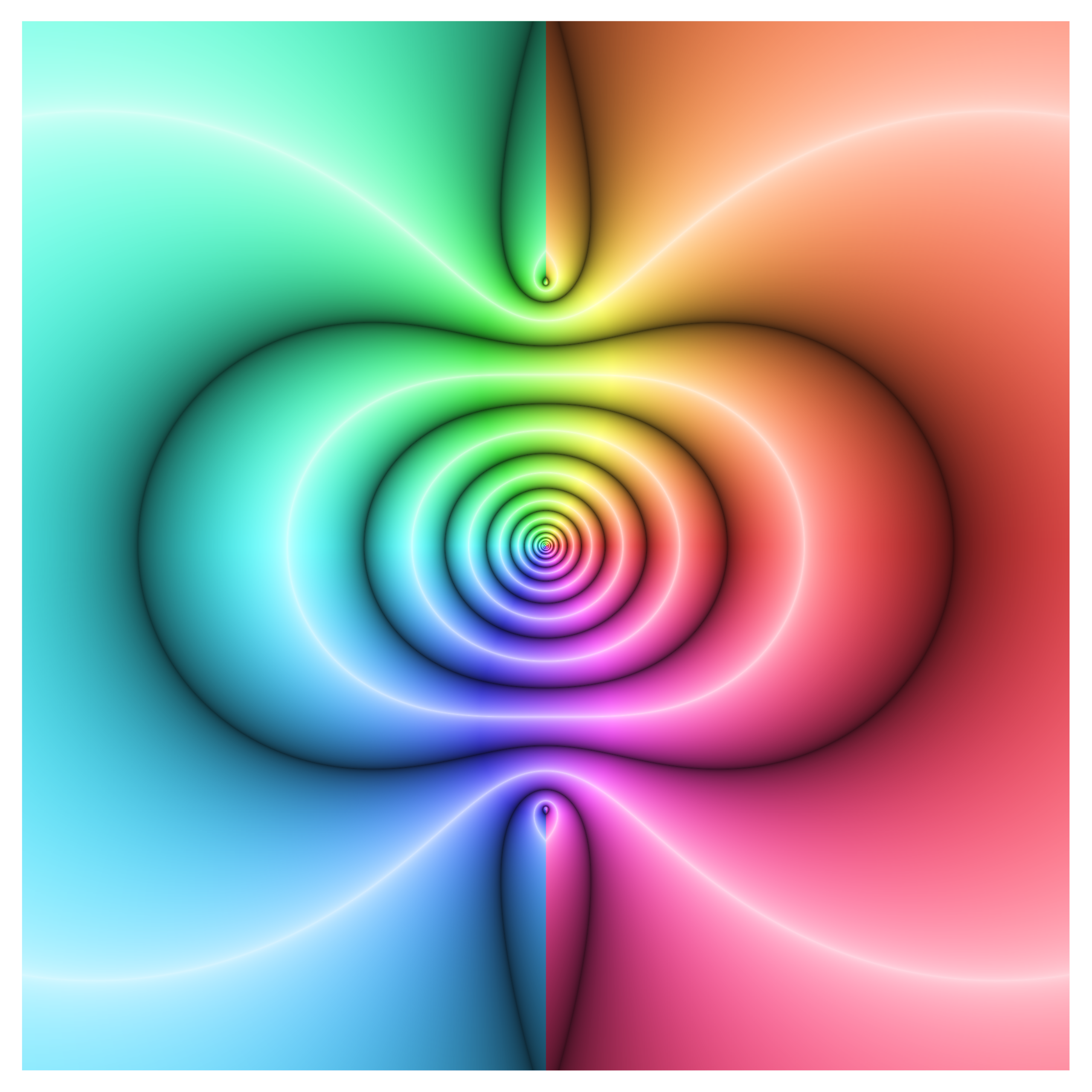
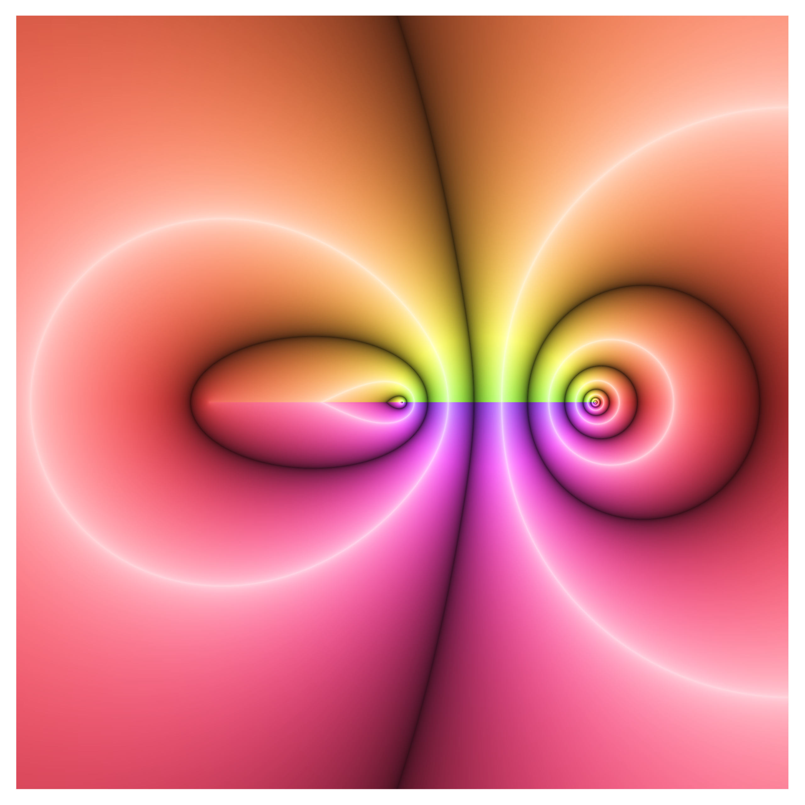
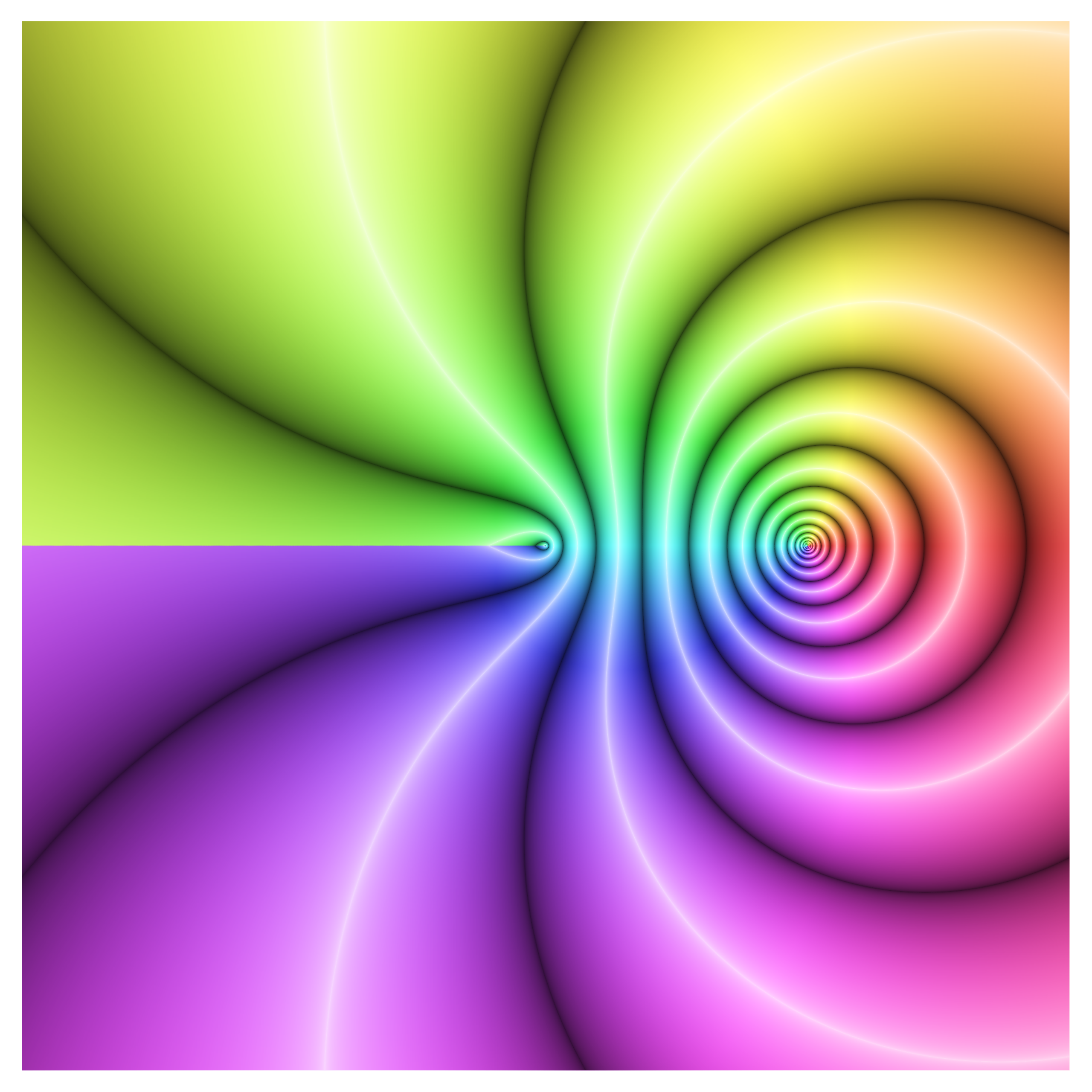
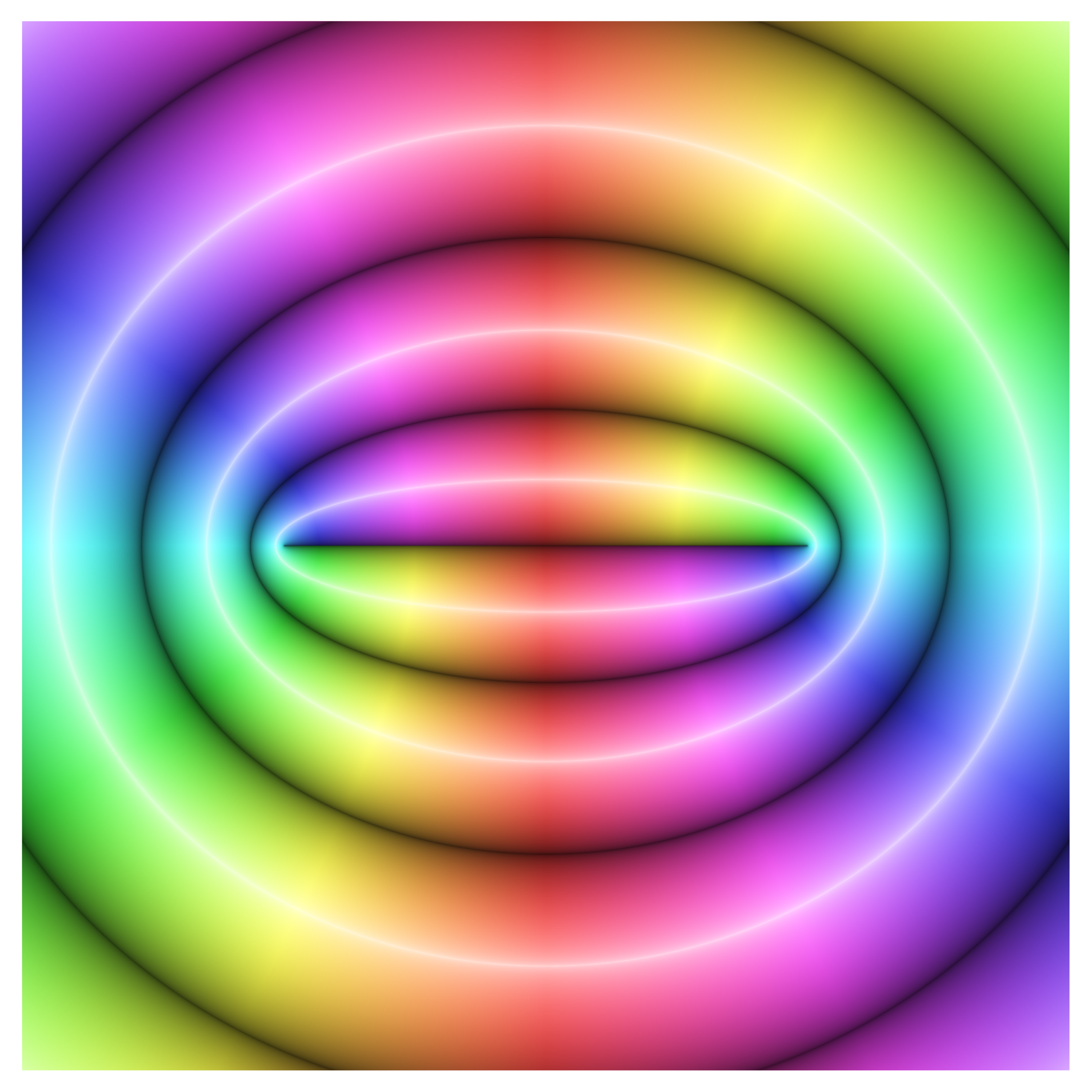
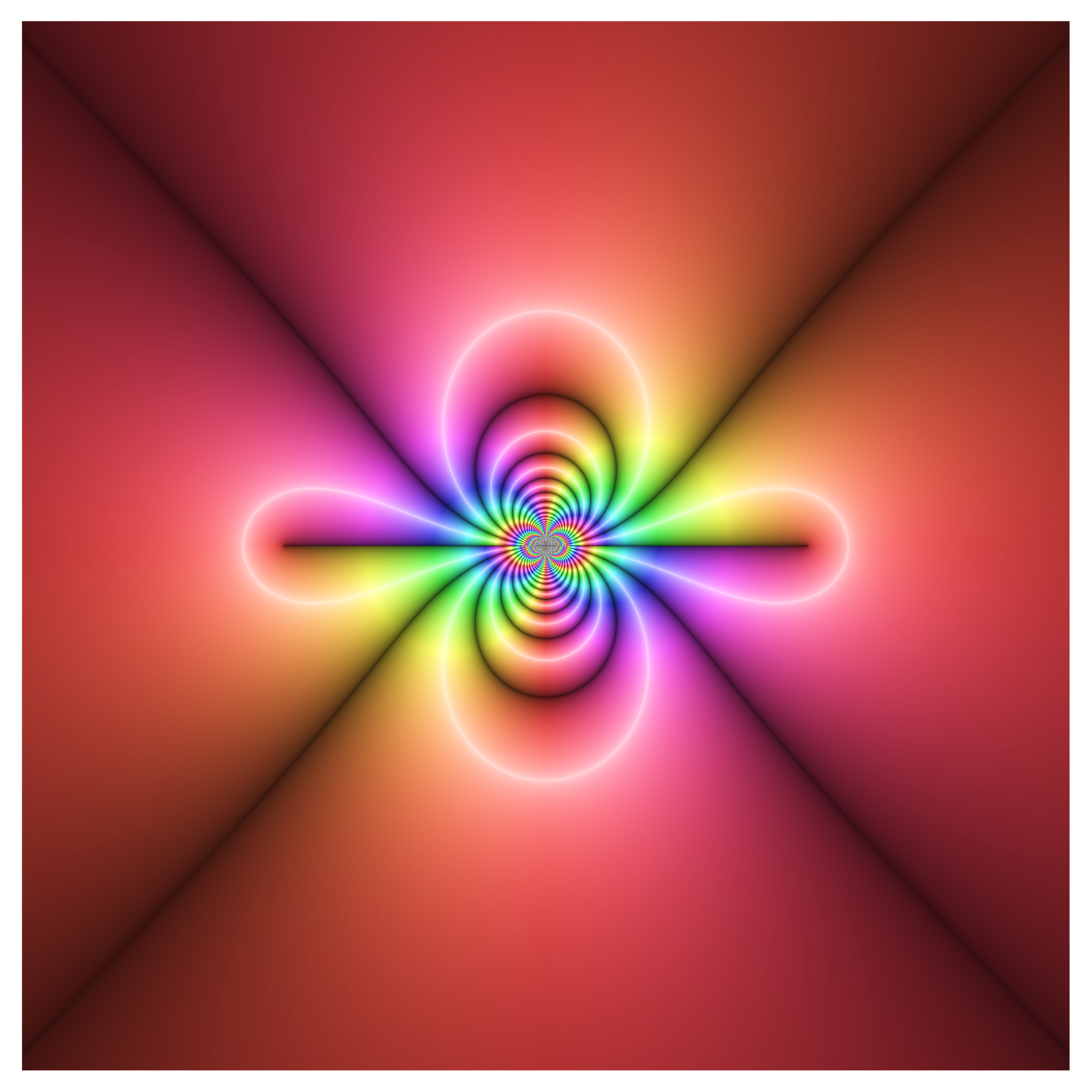
When I saw this image by Claudio Rocchini in undergrad, I immediately started trying to make more like it. The contour lines trace correspond to the level curves of the logarithm of the magnitude of the function at that point. Hues move red-green-blue counter-clockwise, so converging contours indicate either a zero or pole. The order of the zero or pole can be determined by the orientation of the color and the multiplicity.
A copy of the Mathematica code used to generate these images can be found here.
Click on the thumbnails for large versions.
These images show the monomials z, z^2, and z^3.
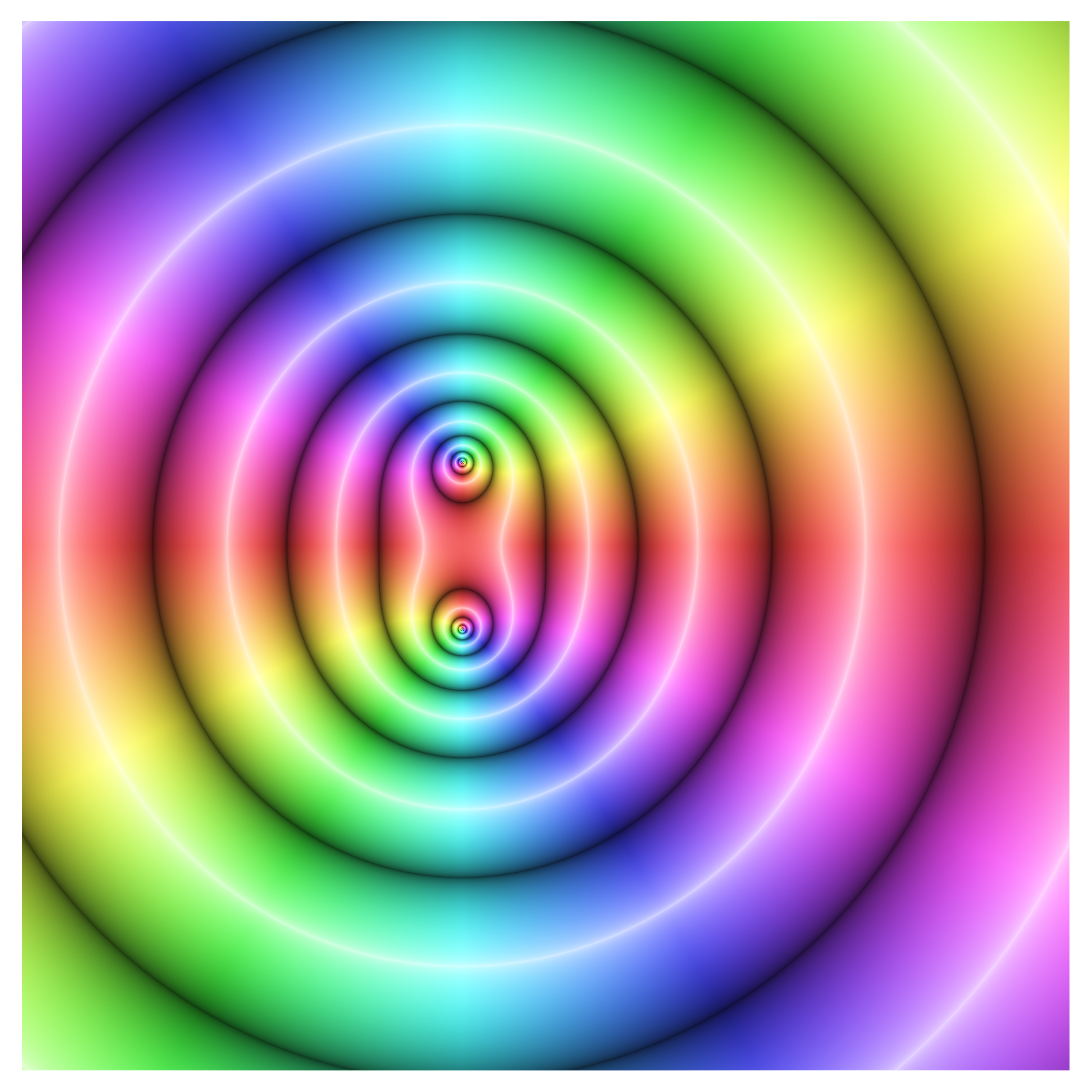
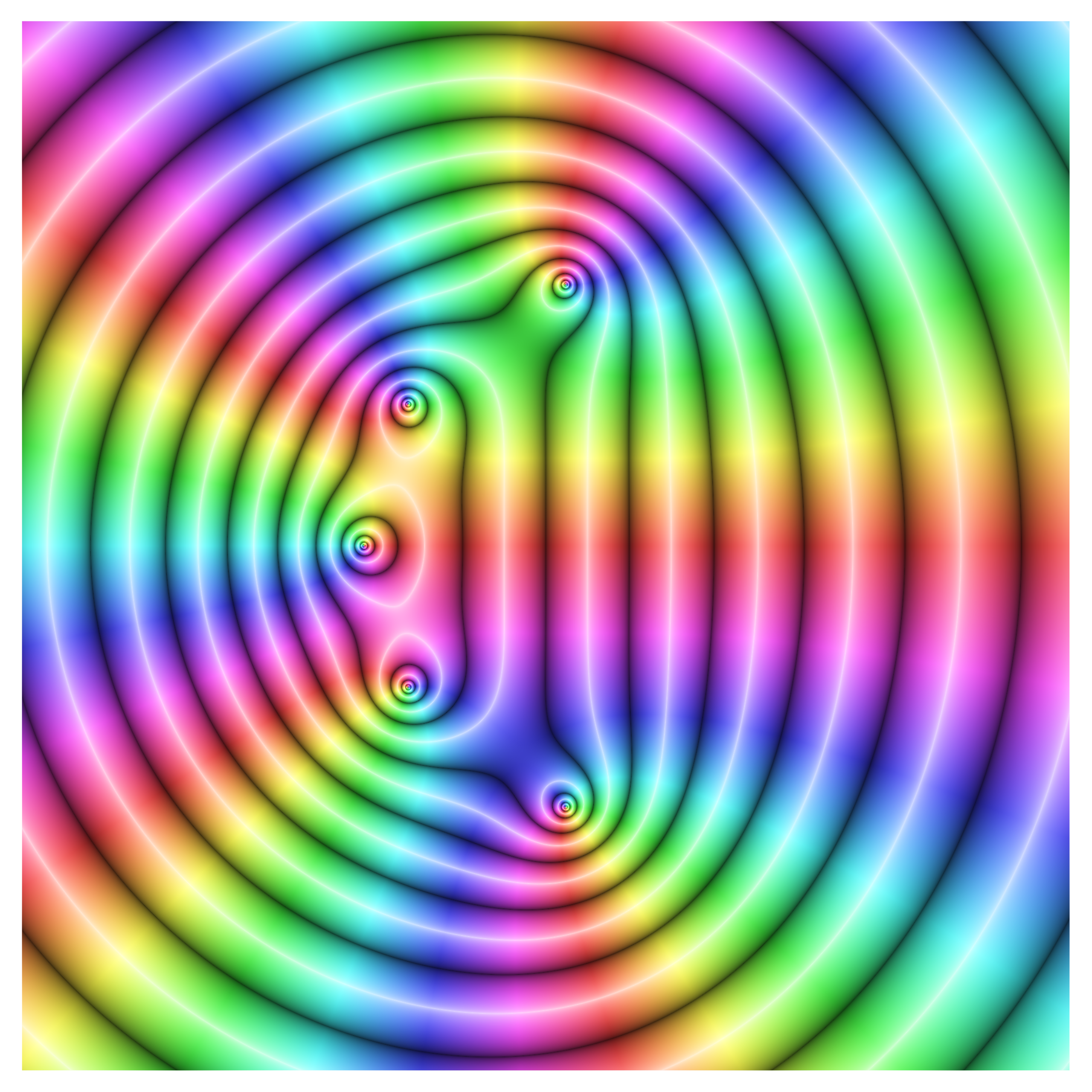
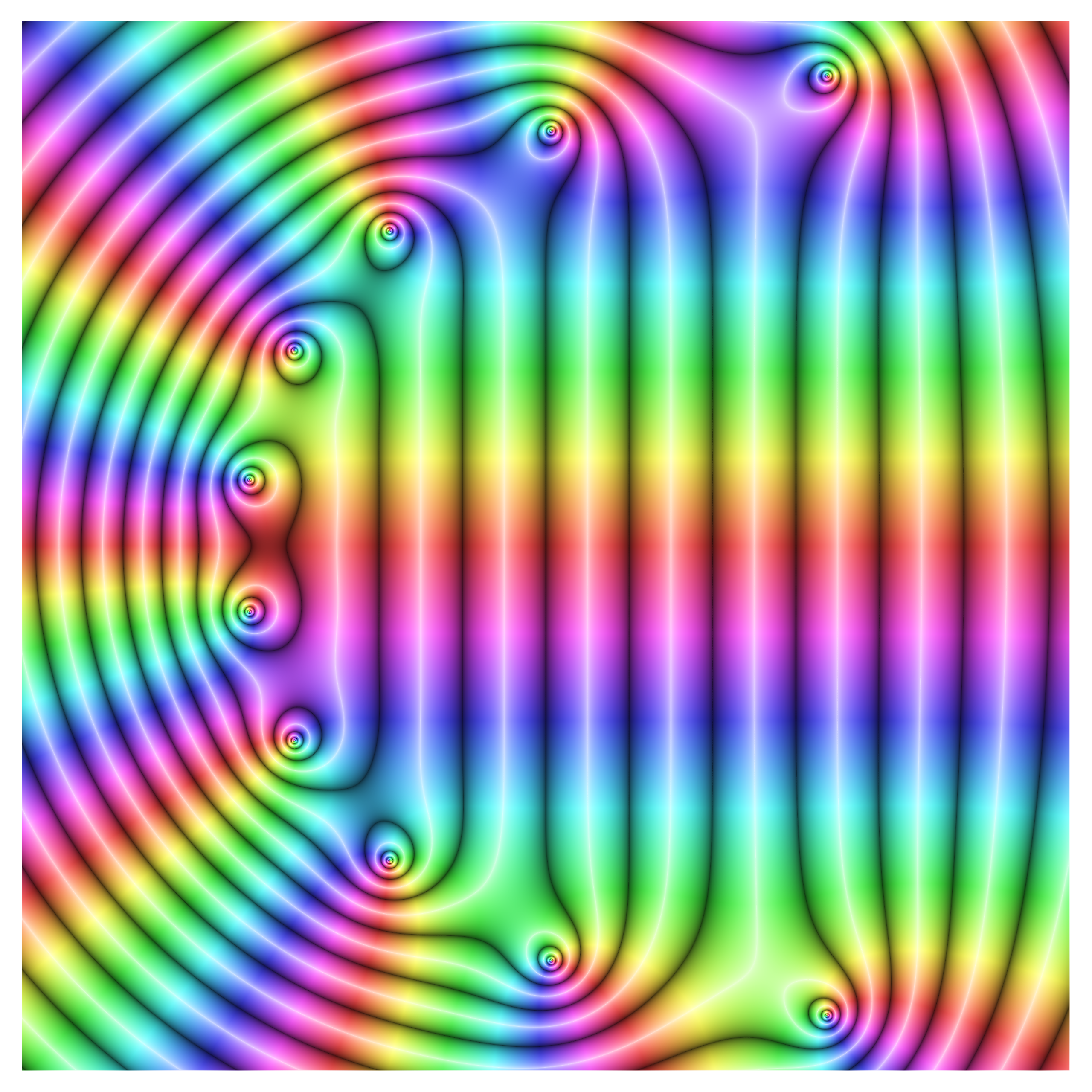
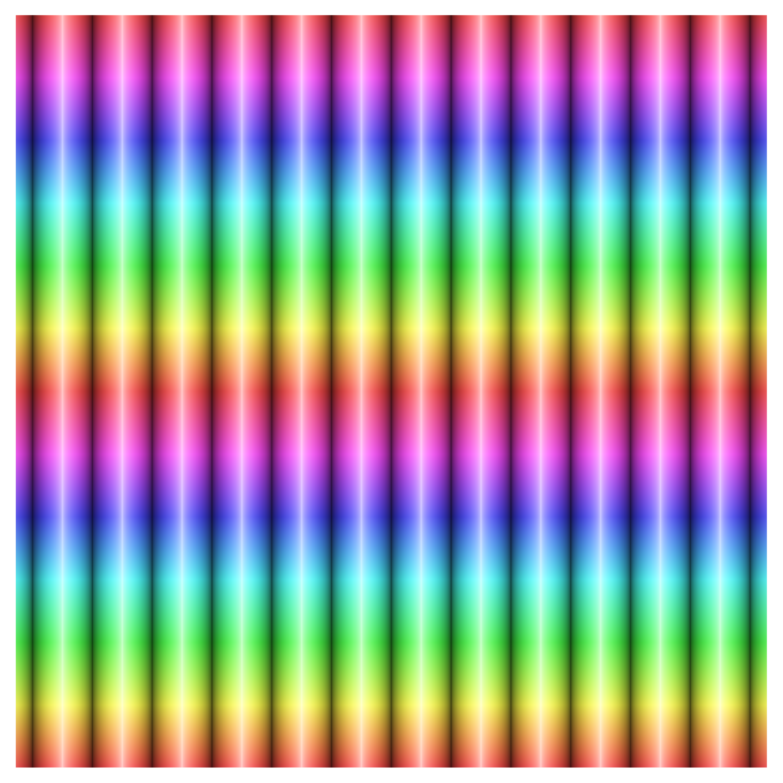
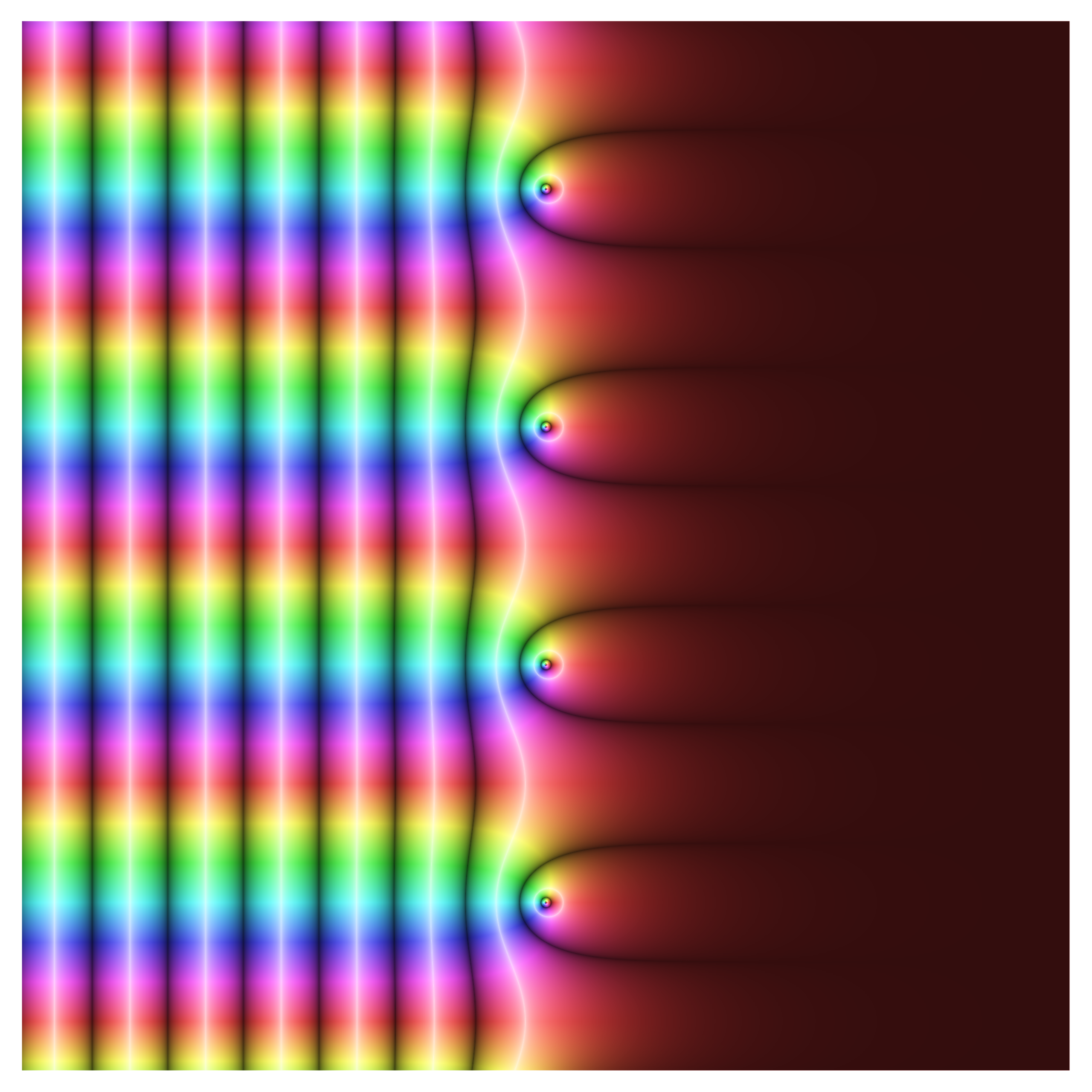
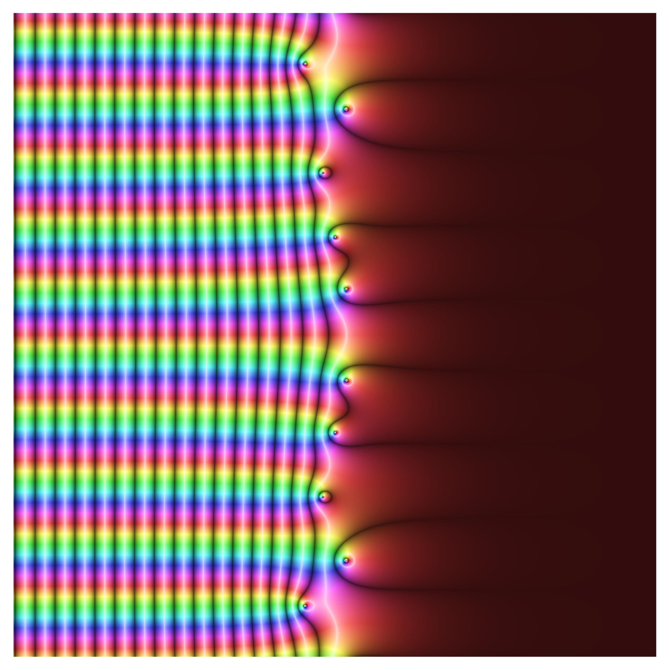
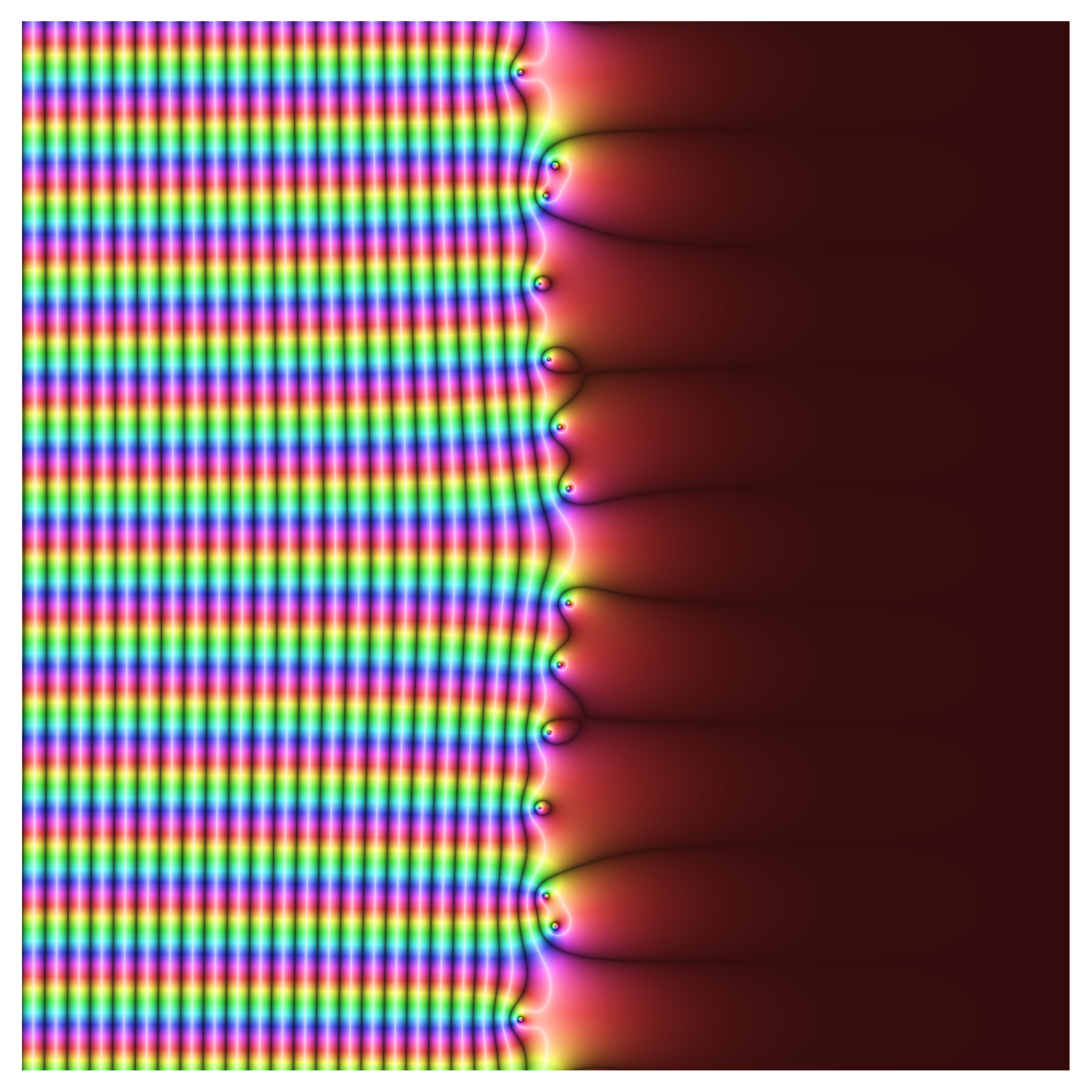
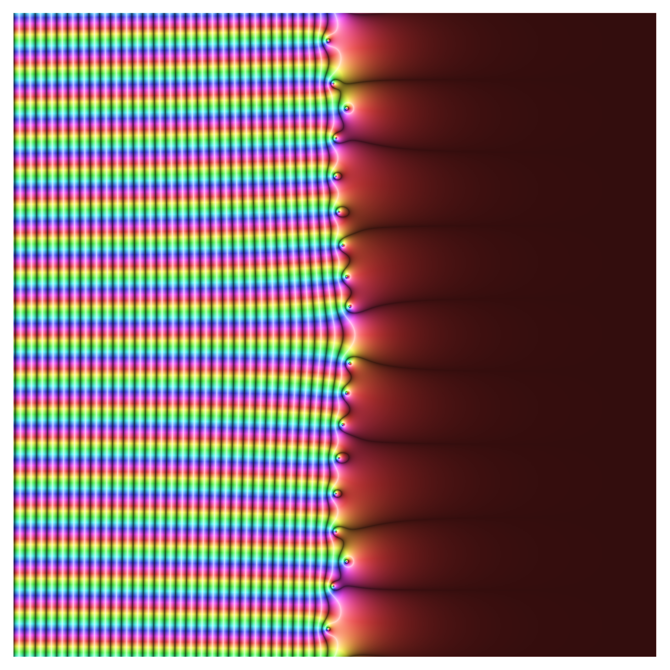
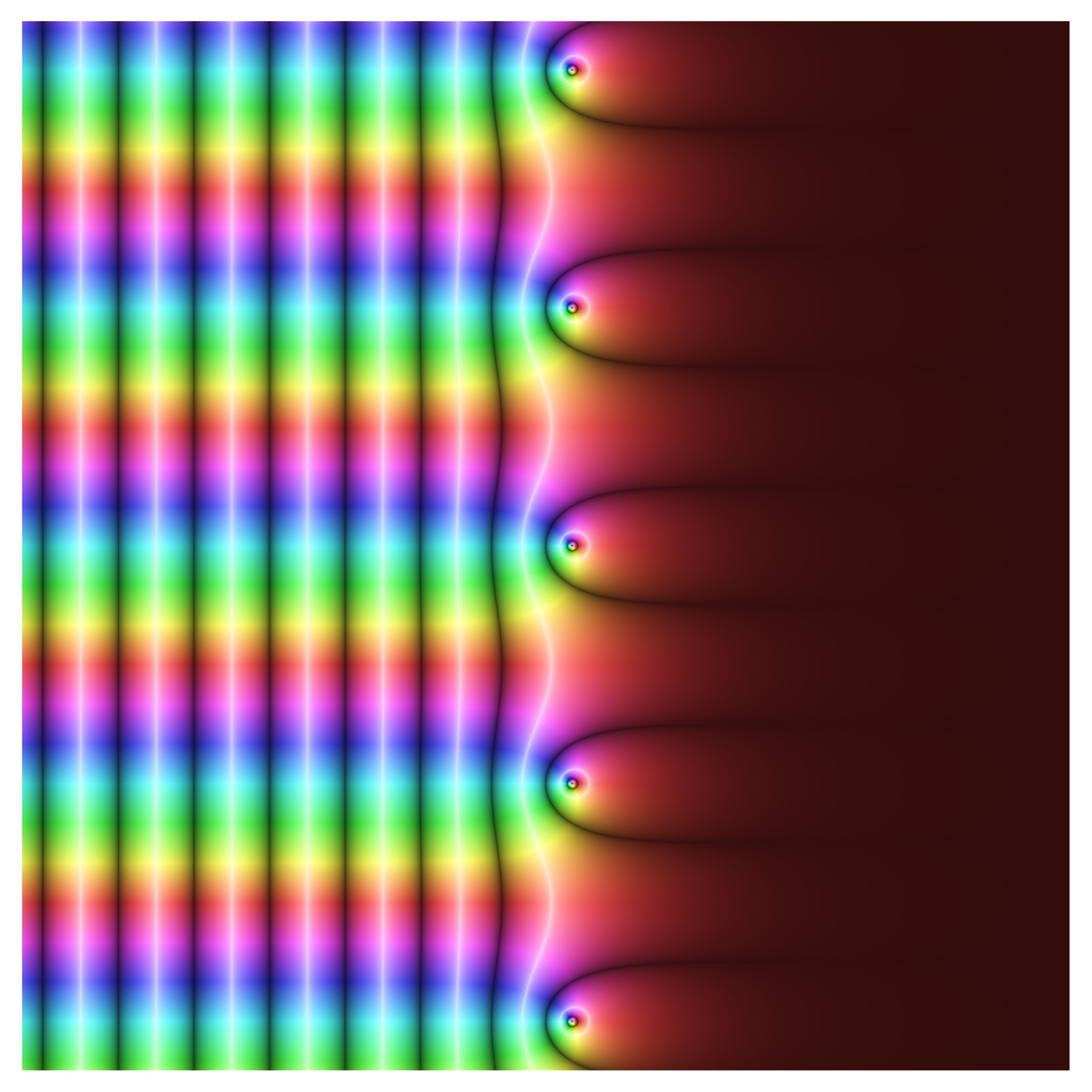
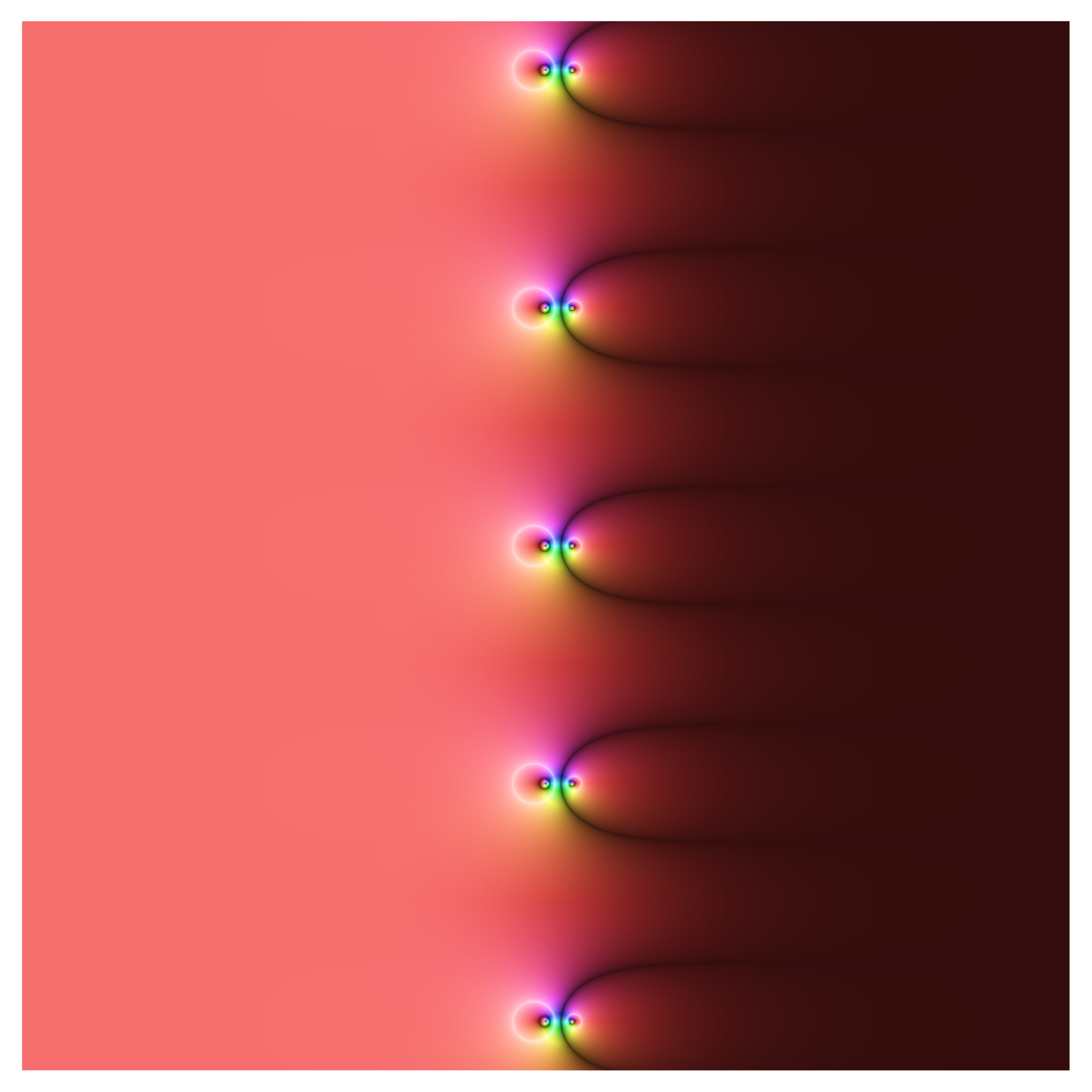
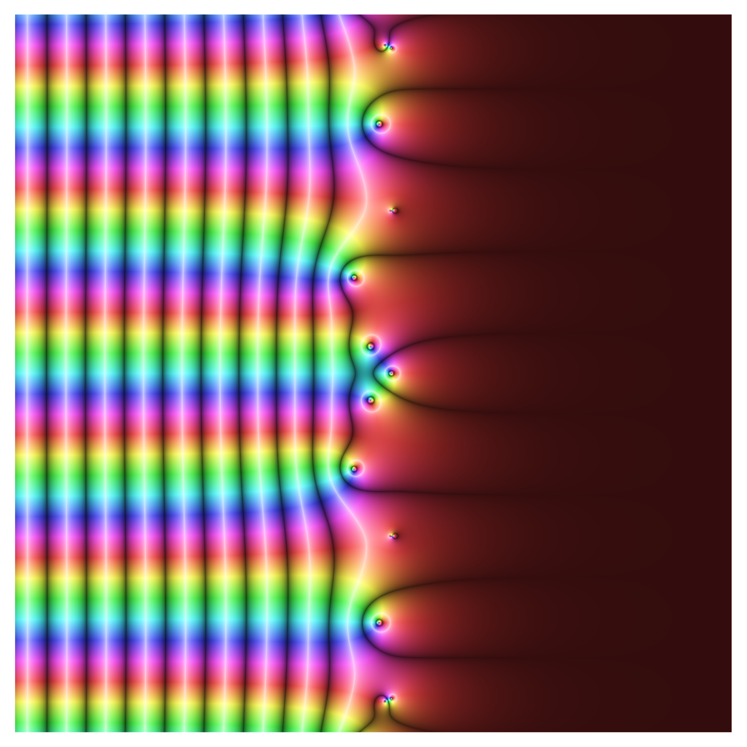
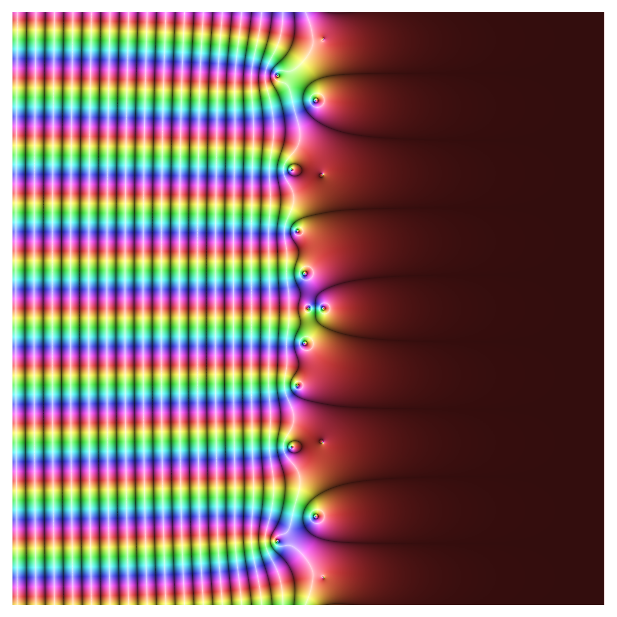
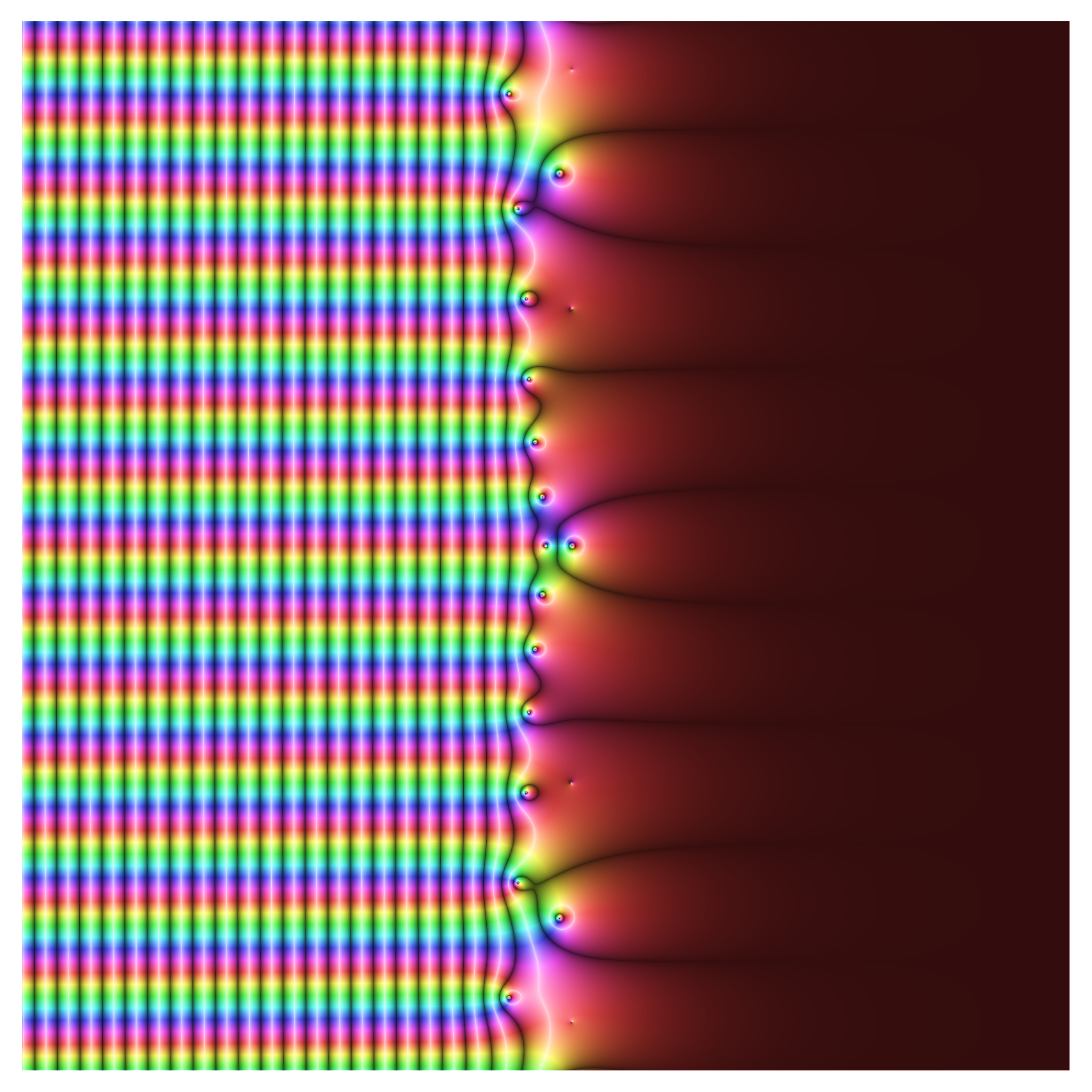
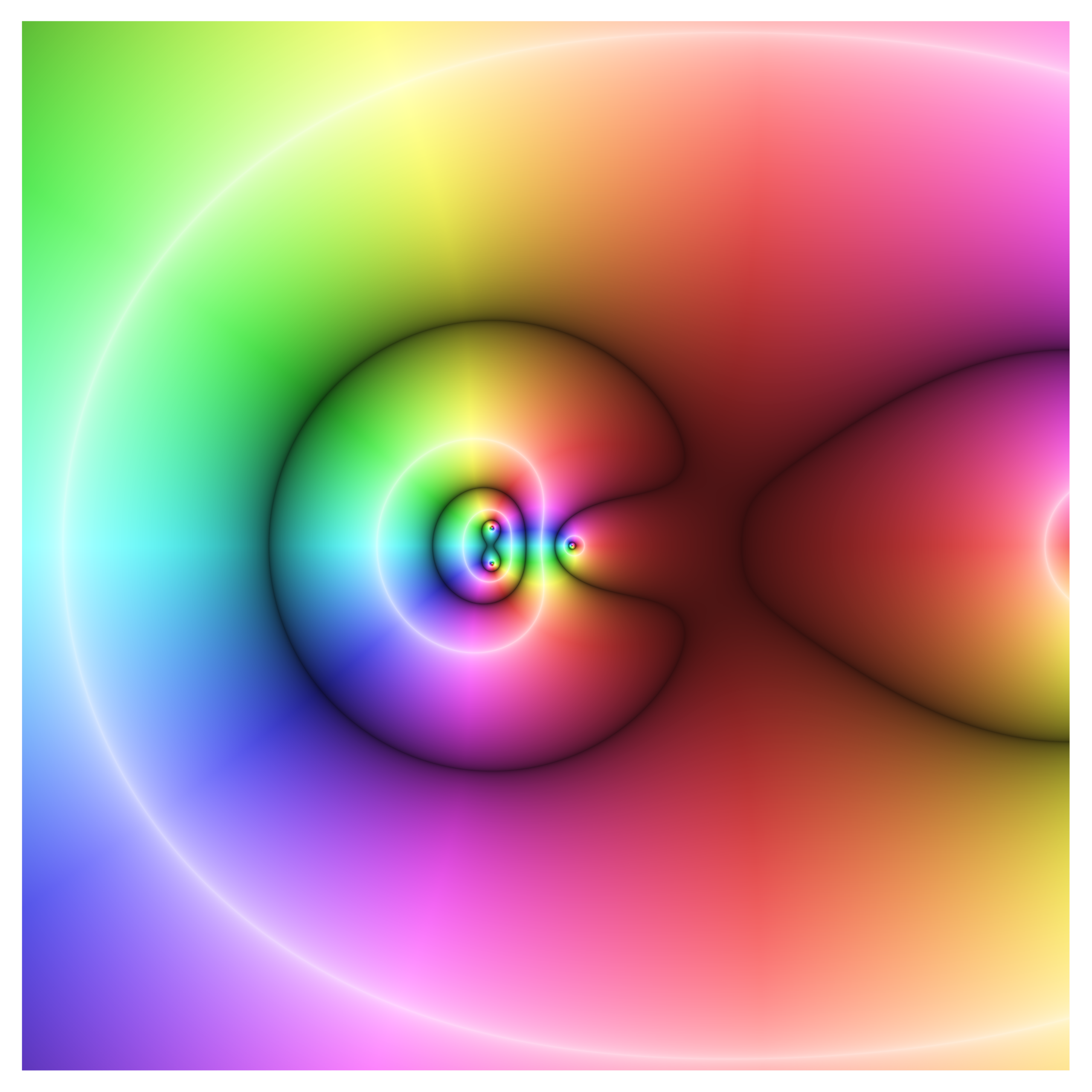
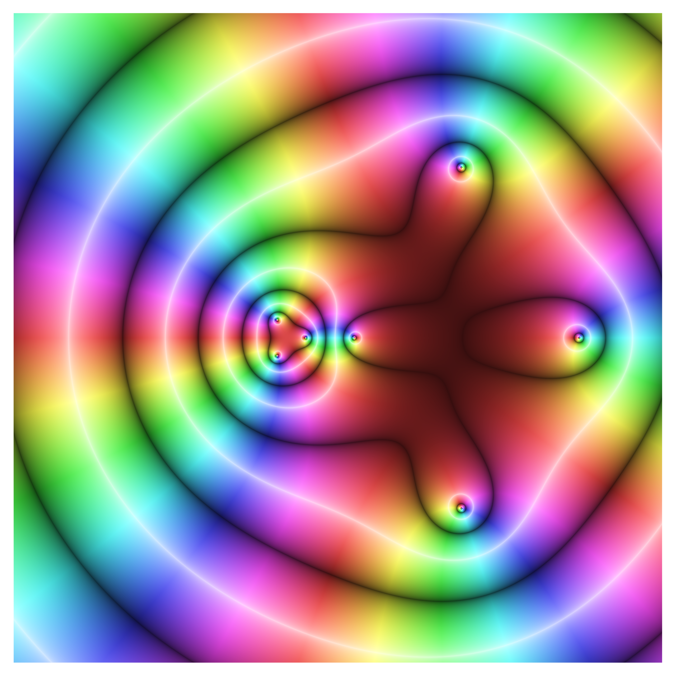
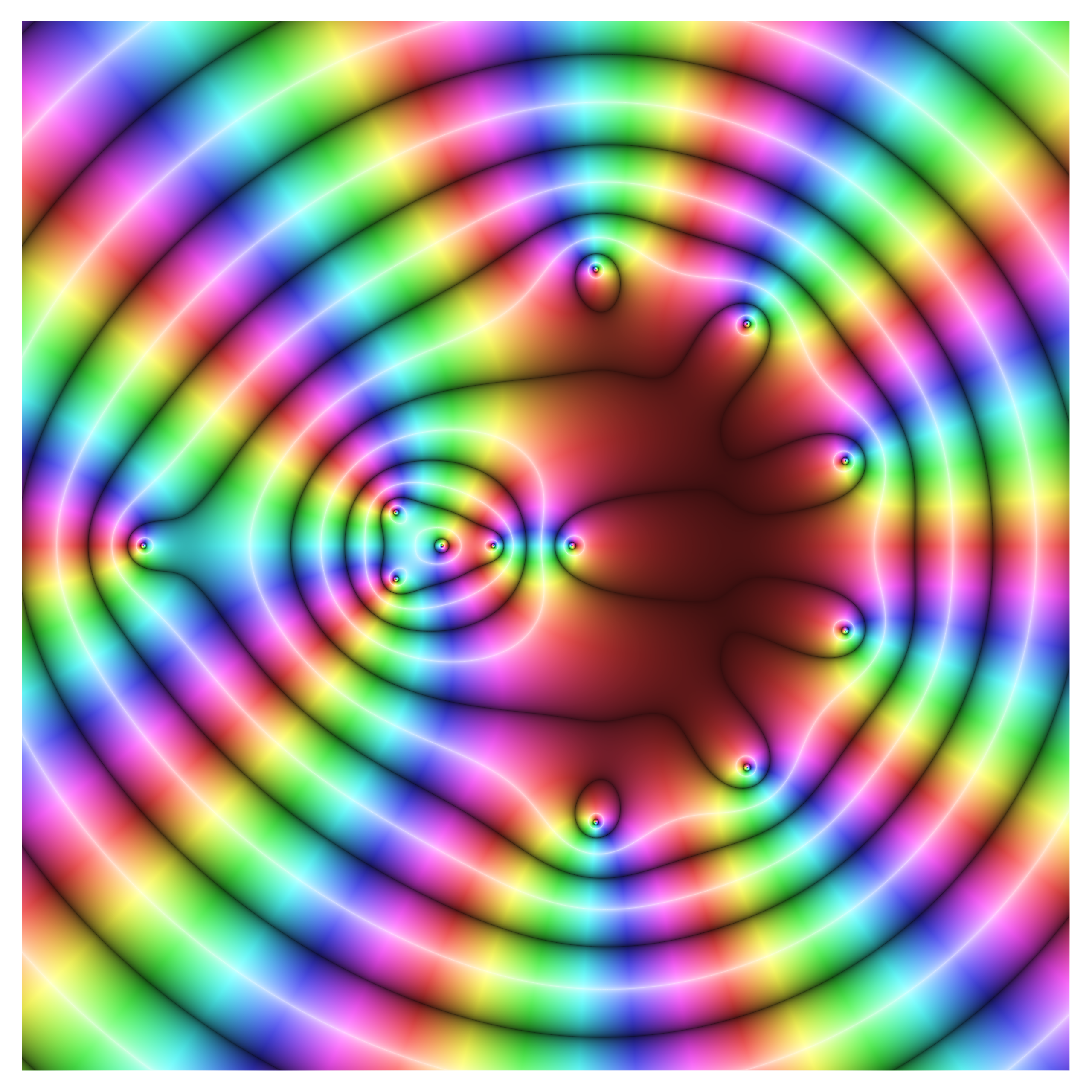
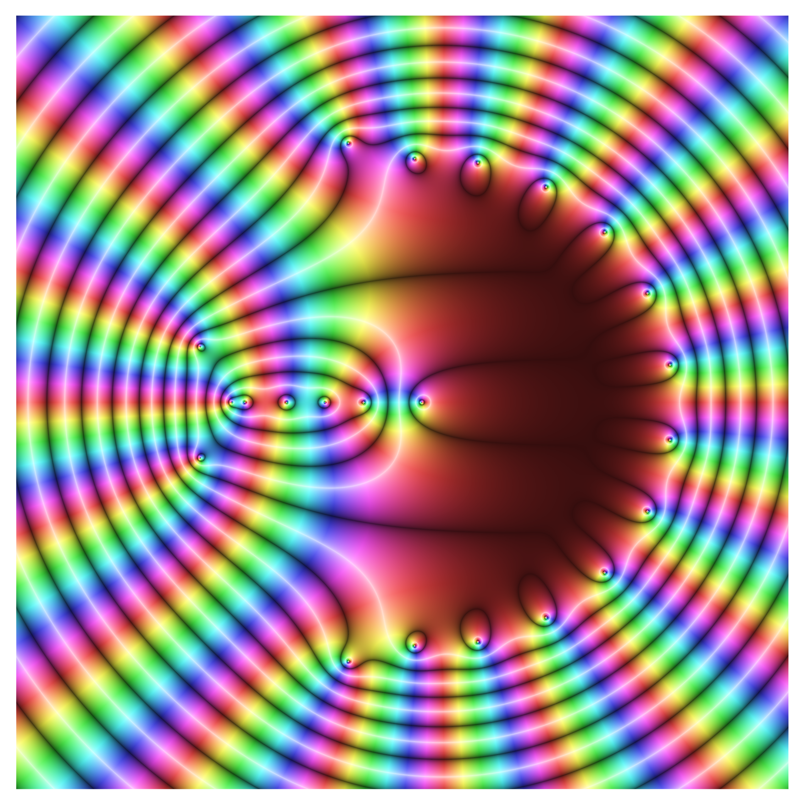
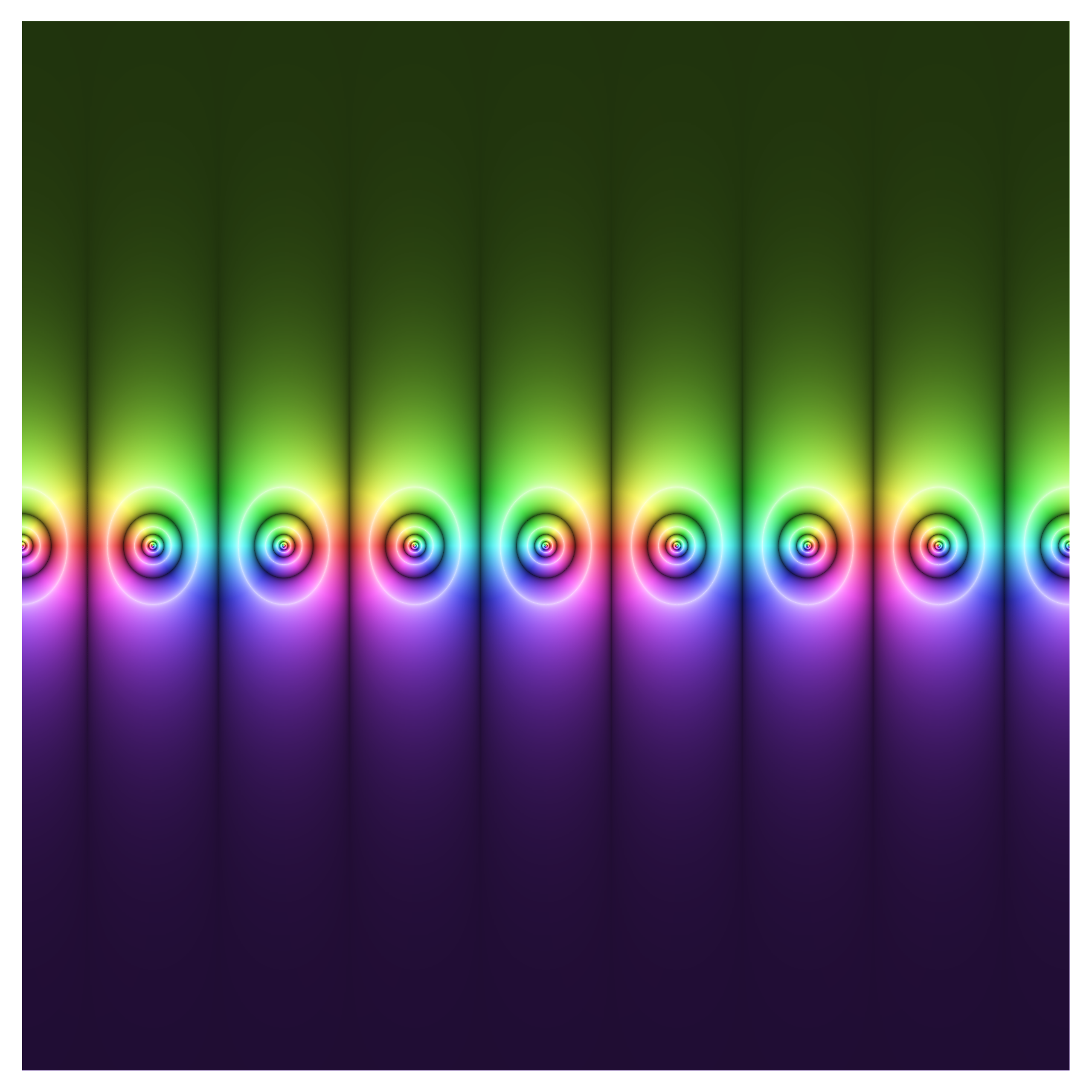
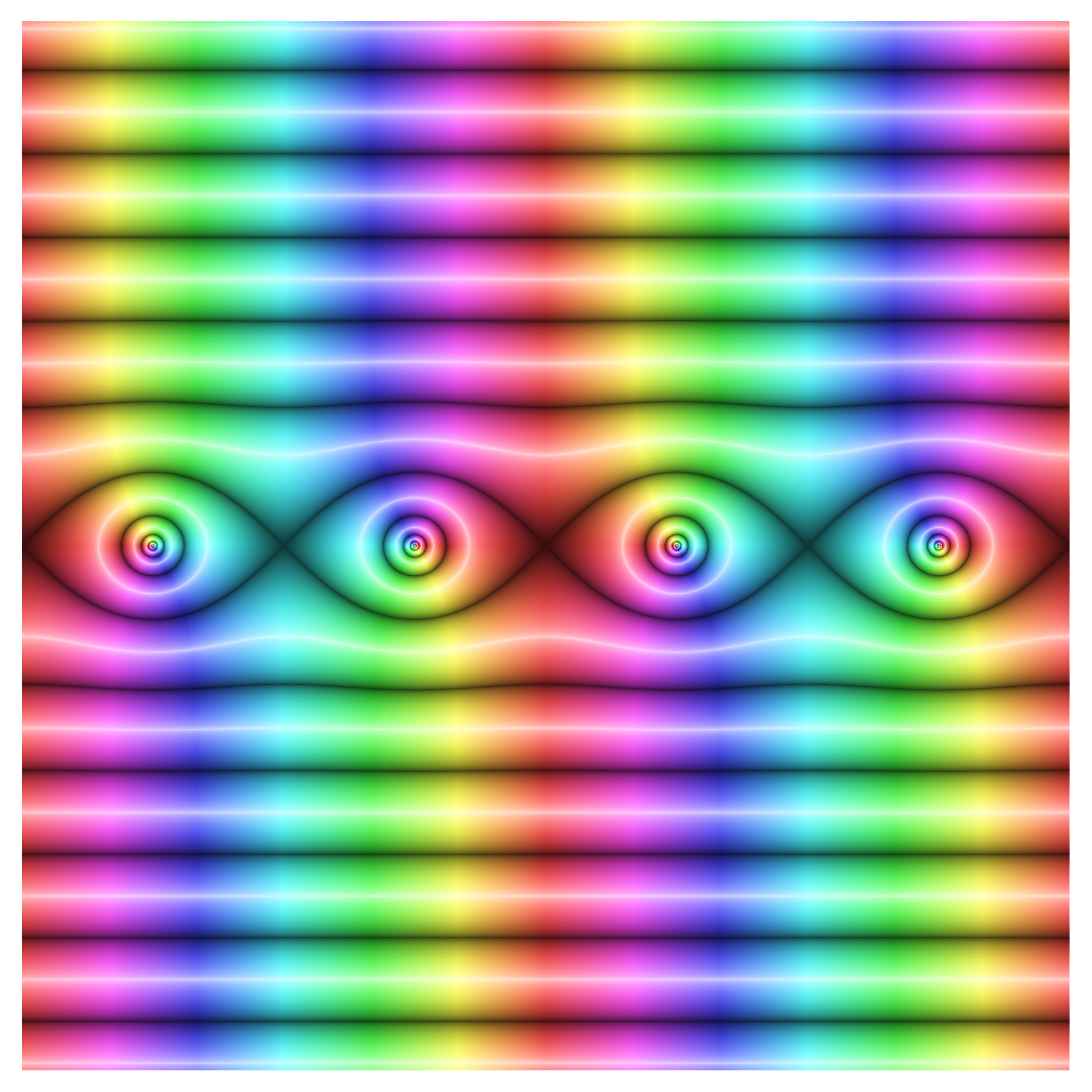
Taylor approximations of the exponential function, compared to the real thing.
Each approximation is a polynomial of higher and higher order, which mean they need more and more roots. On the other hand, the exponential function has no roots. If you fix a finite disk, however, the approximations must converge uniformly on its compact closure. So what happens? The answer is that a corona of zeros form, which move further and further out. As the number of terms in the approximation goes go infinity, the zeros all escape to the point at infinity, where the exponential function has an essential singularity.

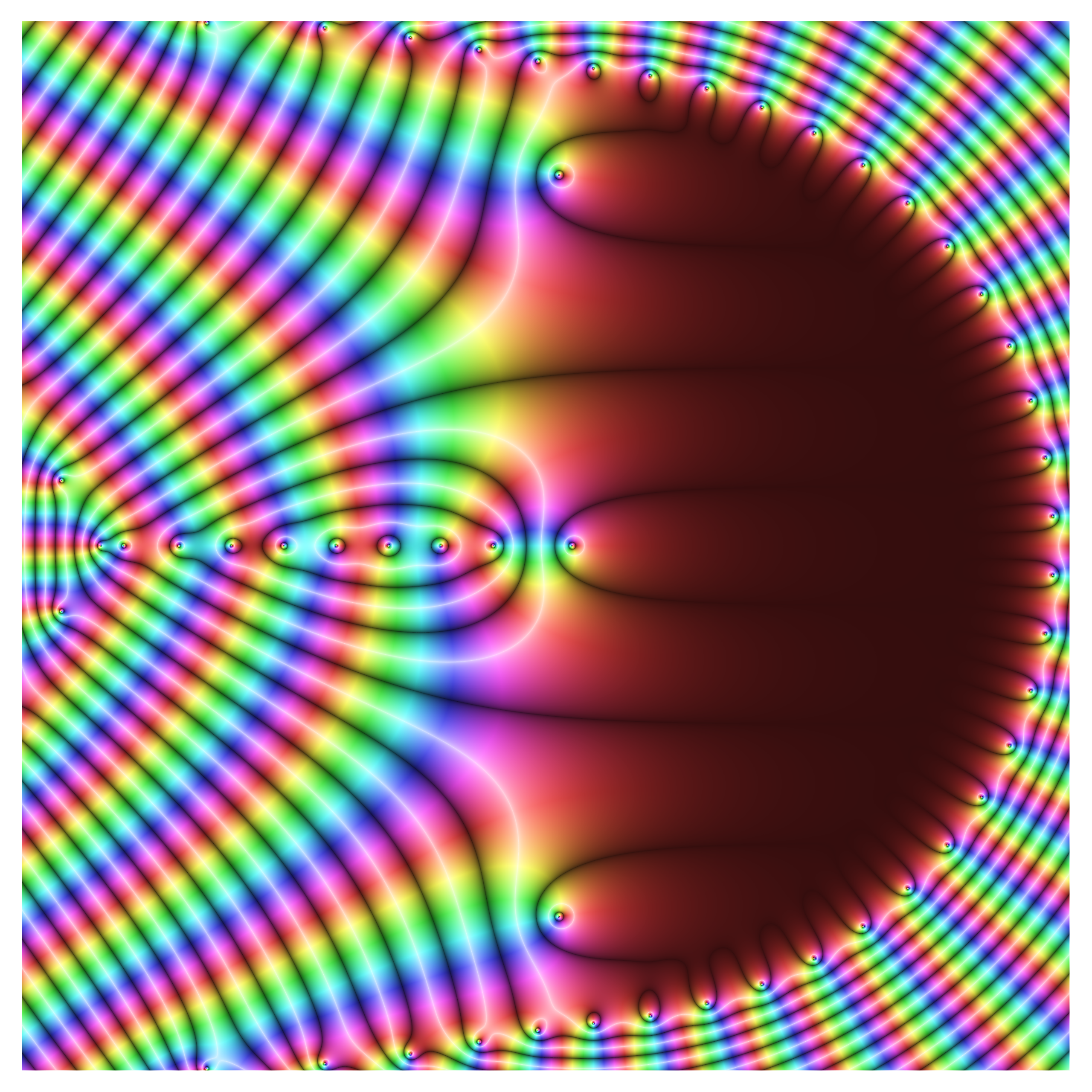
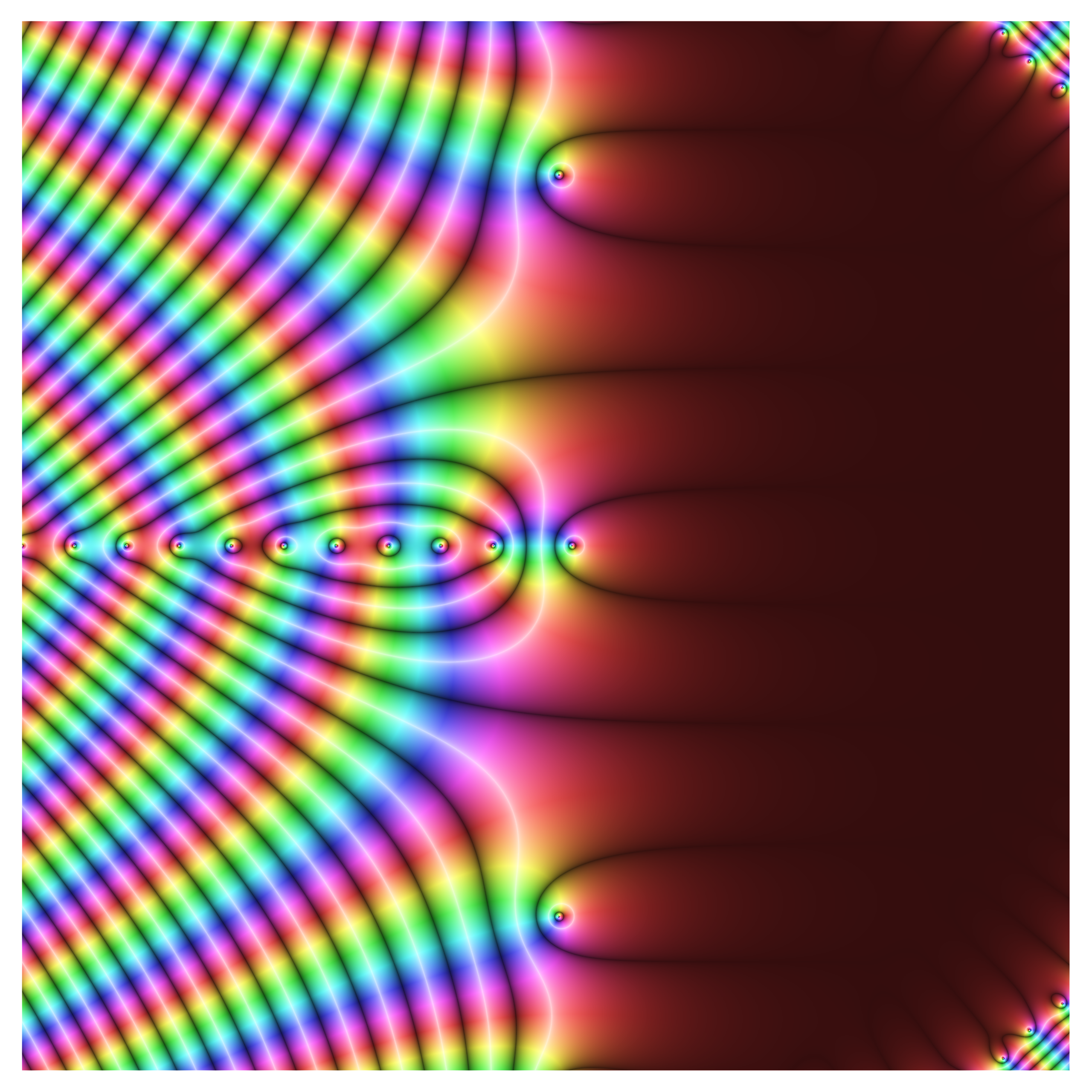
Dirichlet series approximations of the zeta function, compared to the real thing. Convergence only occurs for real values greater than 1, so the zeros in the critical strip are not in the region of convergence.

Eta function approximations of the zeta function, compared to the real thing. Convergence only occurs in the right half plane, so the zeros in the critical strip are in the region of convergence.
Laurent approximations of the zeta function, compared to the real thing.
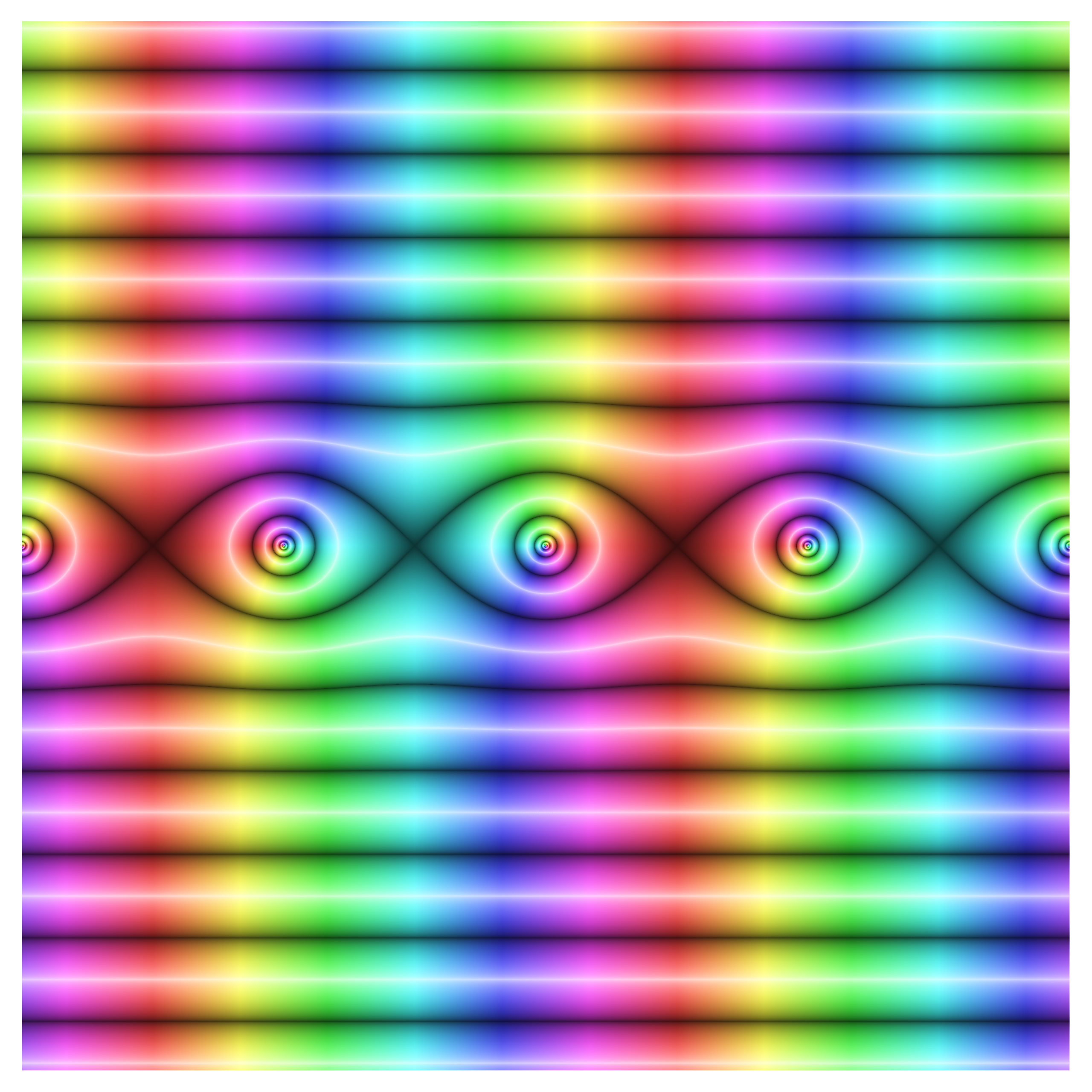
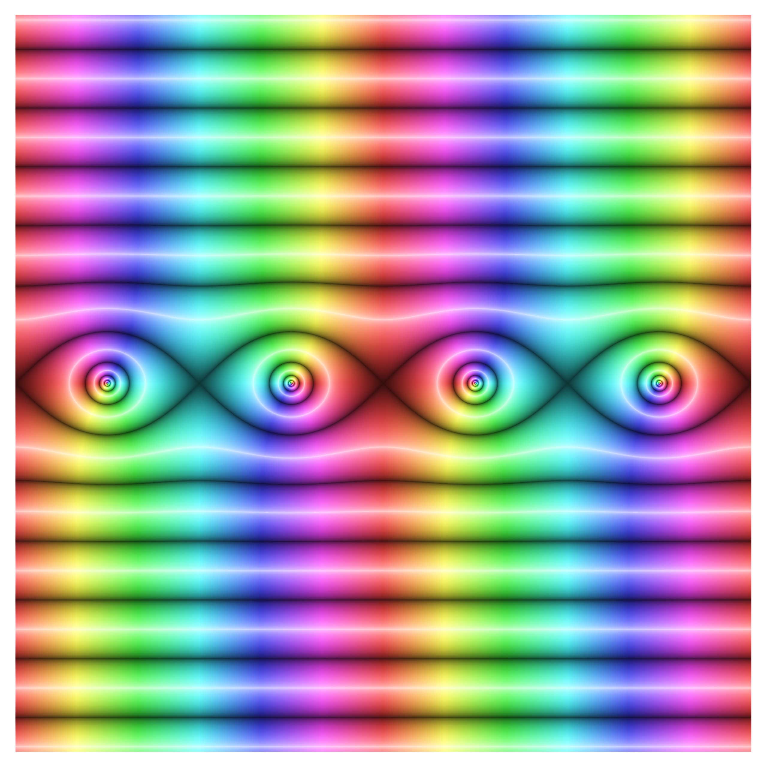
Trigonometric functions sine, cosine, tangent, and secant.
Branches of inverse trigonometric functions arcsine, arccosine, arctangent, arcsecant, and the complex logarithm.
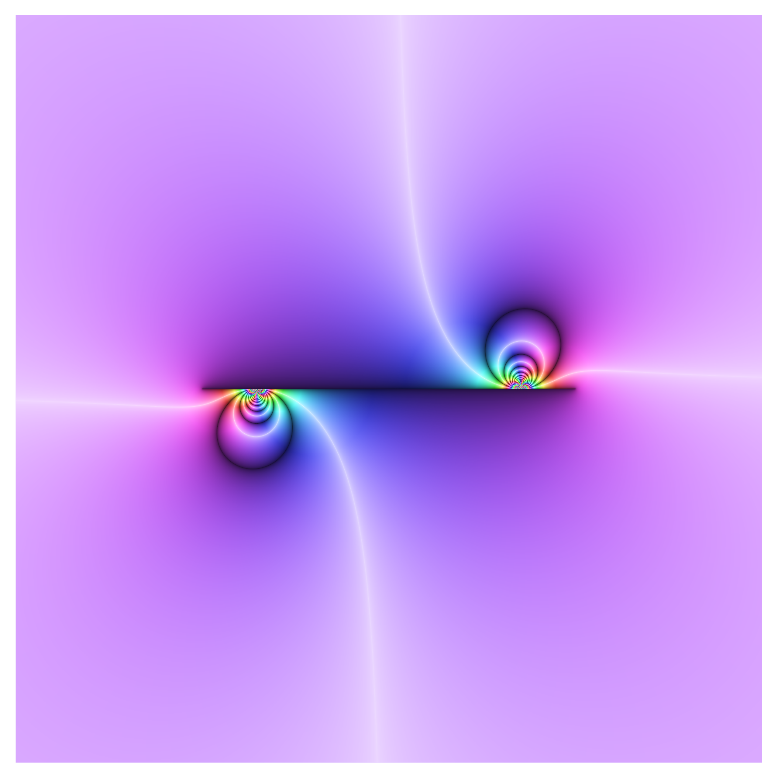
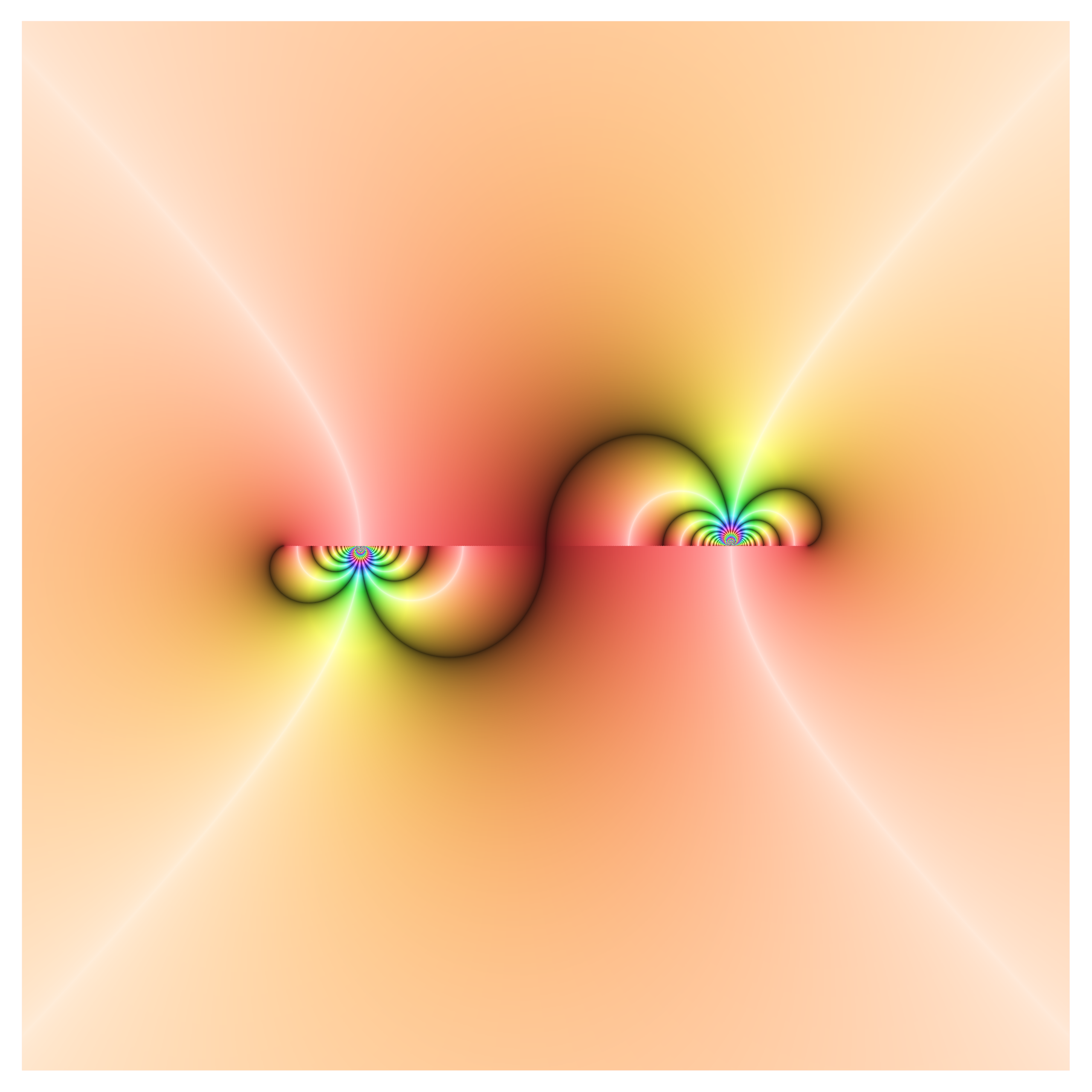
Bounded maps of the slit plane.
It is impossible to construct bounded maps on the entire plane, but you can cut points out in order to make it possible. A simple way is to cut the line [-1,1]. The first image can be thought of as a function on a two-sheeted Riemann surface, where the slice is actually a fold which transports you to the other sheet. On this sheet the function is bounded in magnitude by 1, on the other sheet it is unbounded.
The second image is composed with an infinite-to-one covering of the unit disk. The other images use conformal maps to slide the function around the cut.
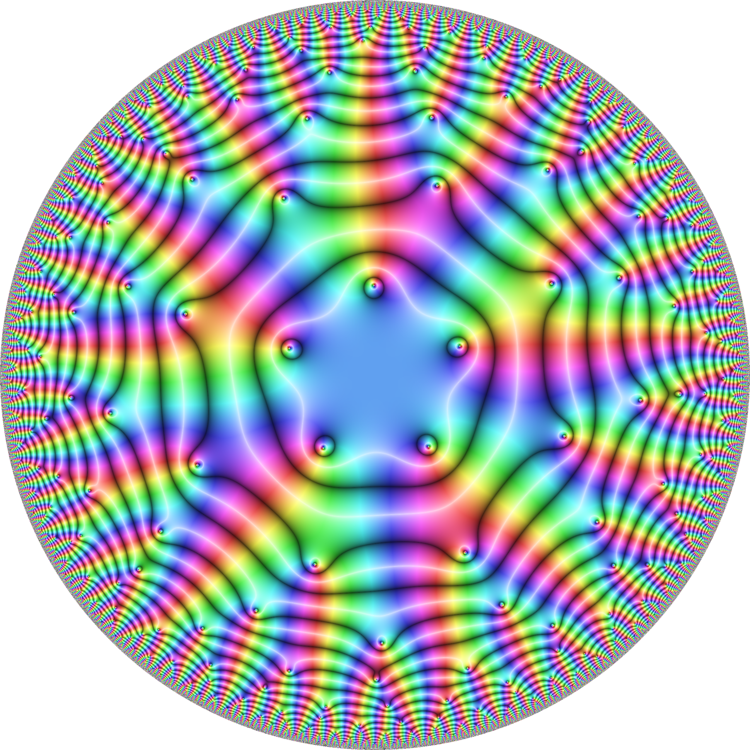
Some maps on the unit disc, including lacunary series. The first is a bounded, infinite-to-one map.
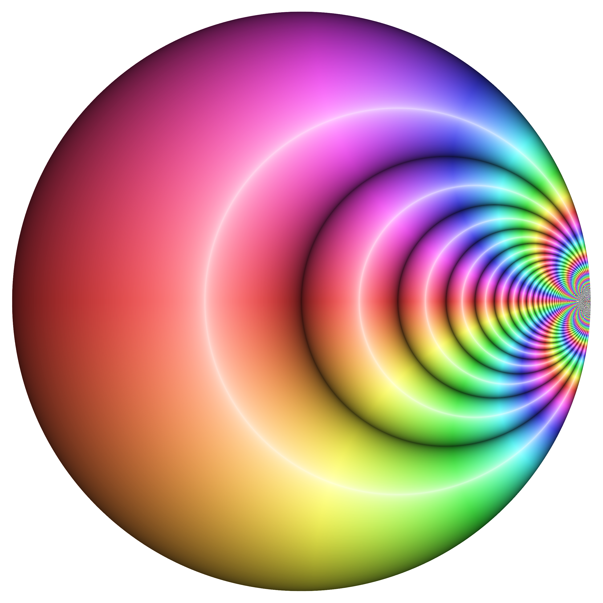
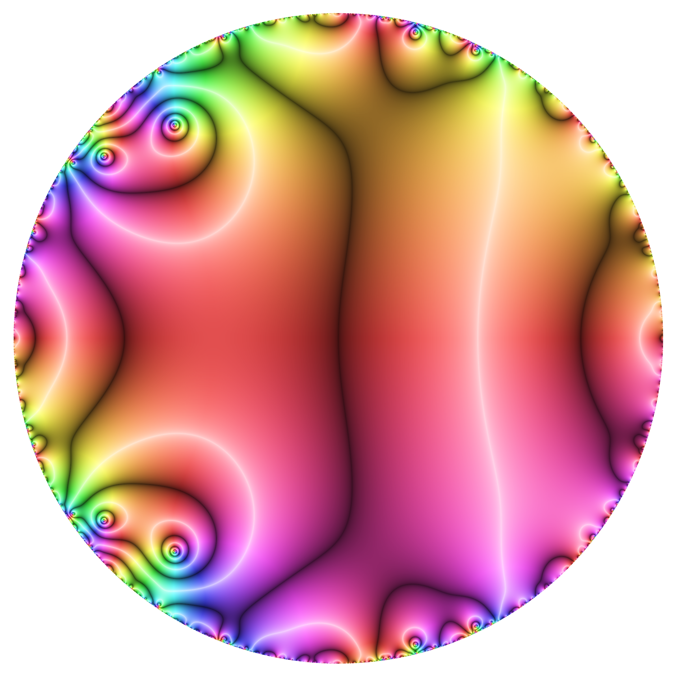
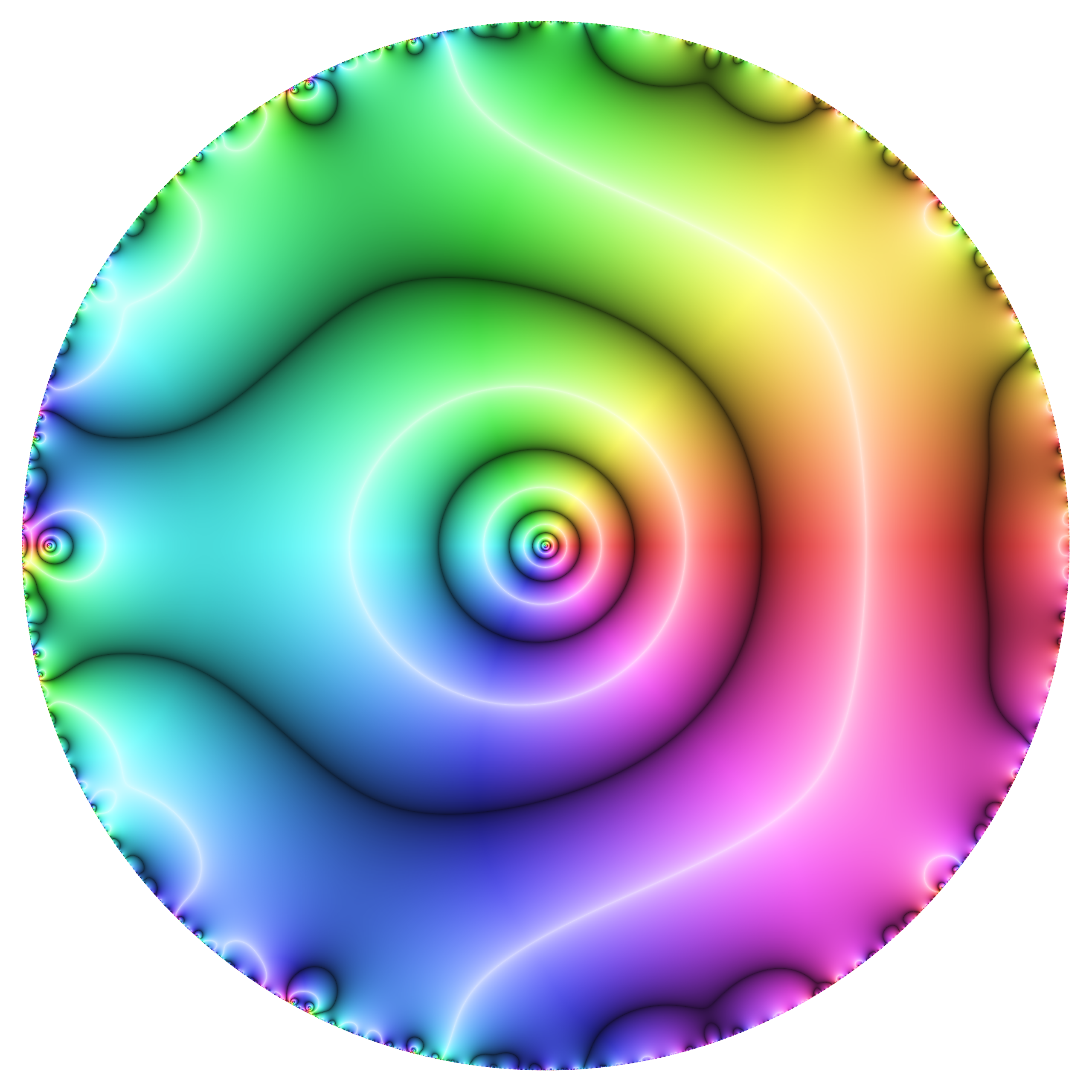
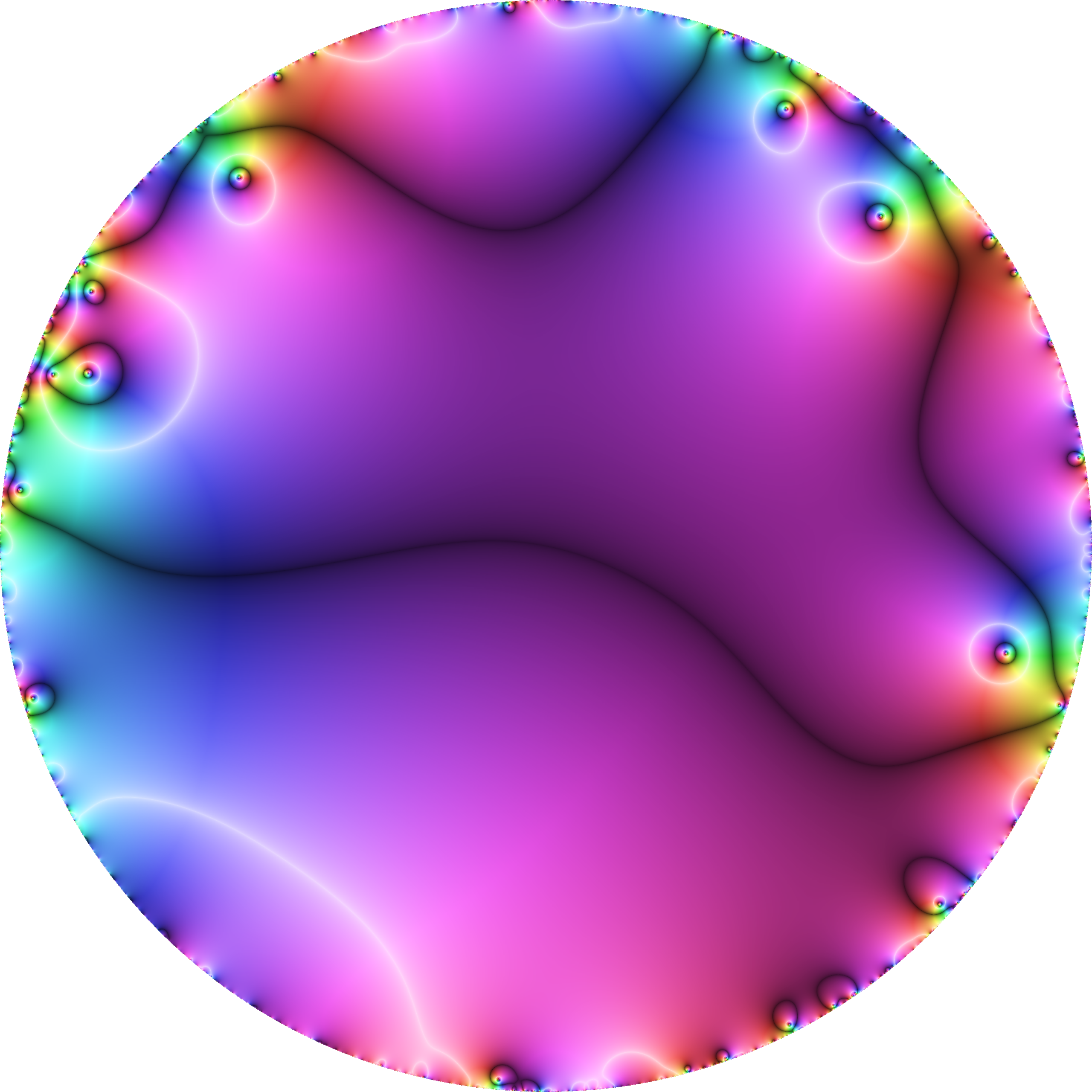
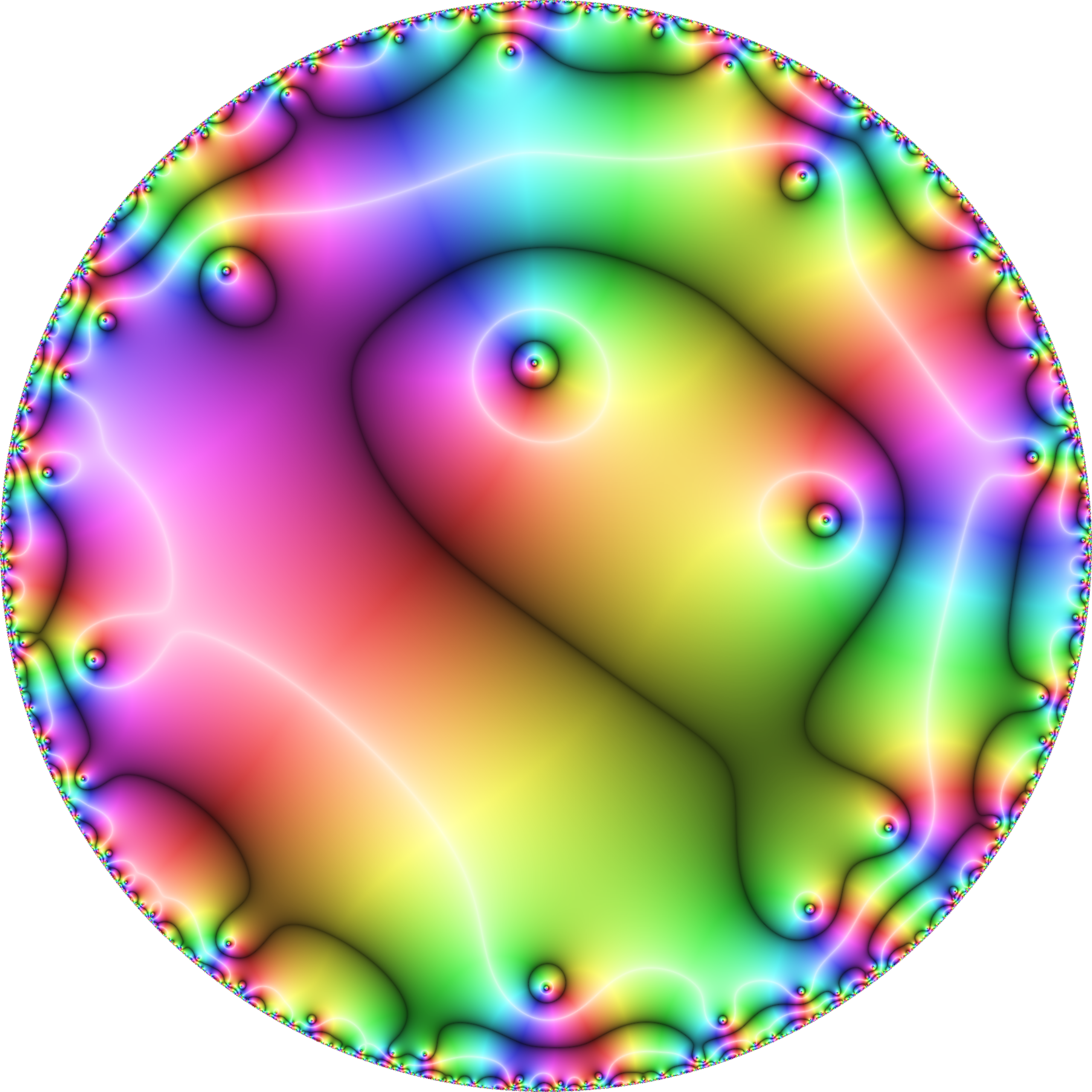
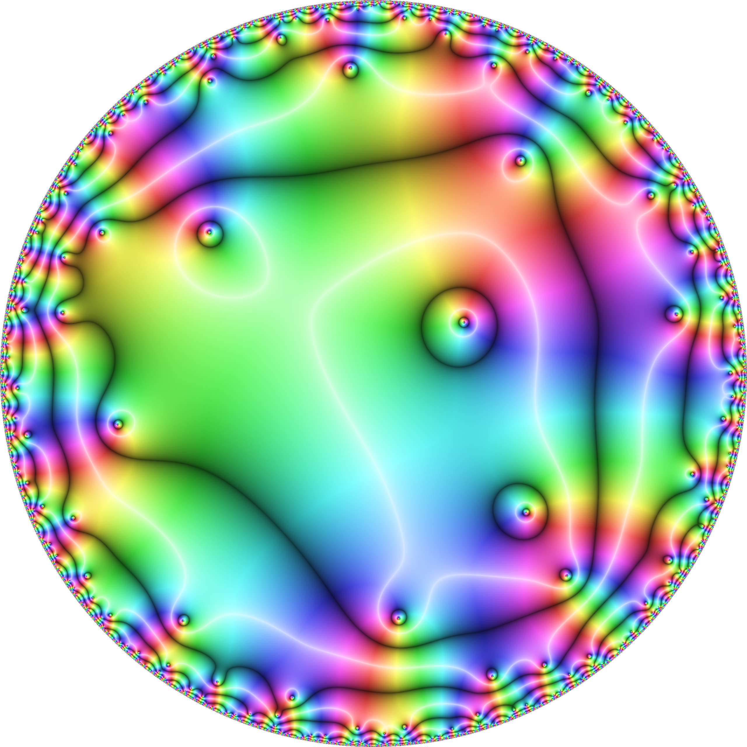
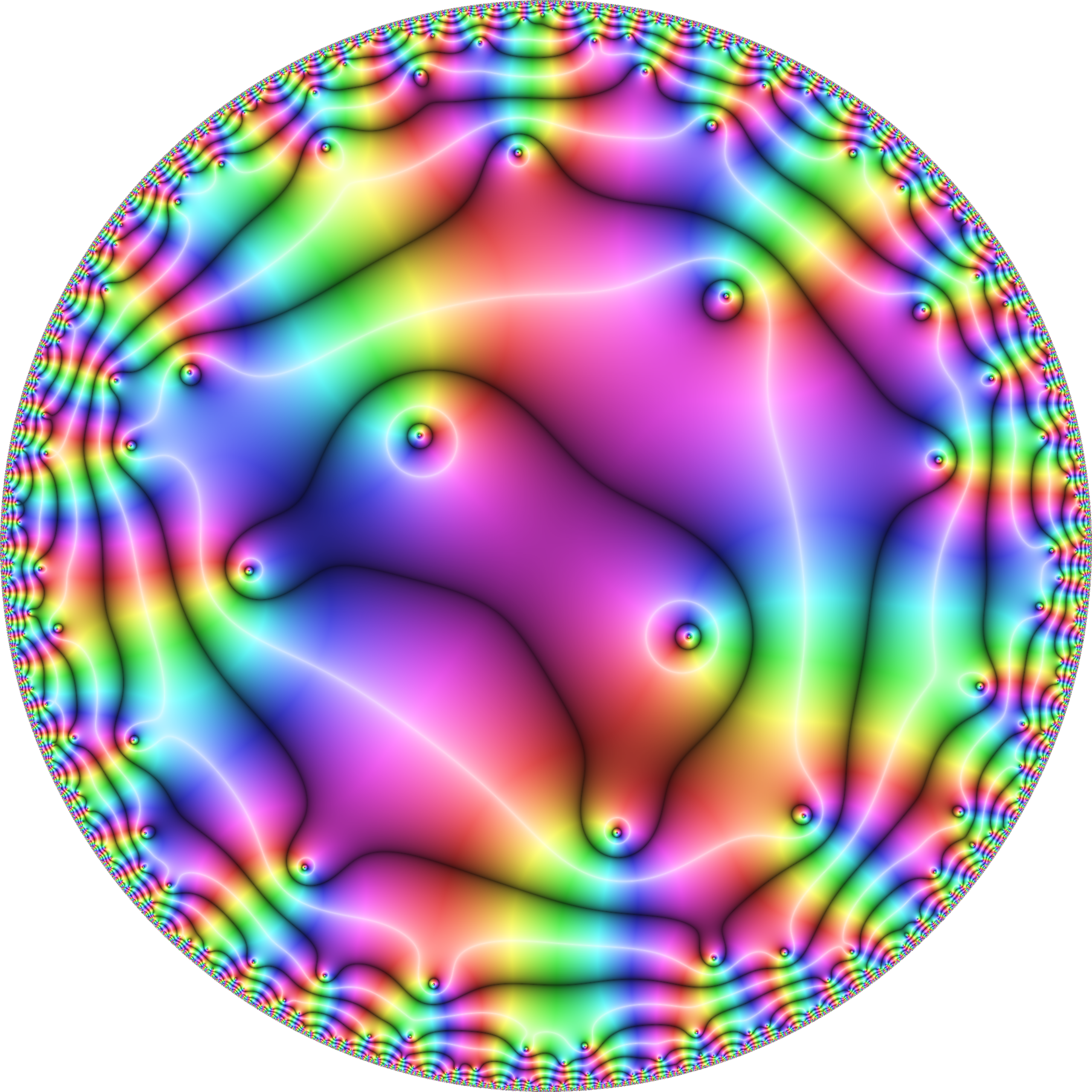
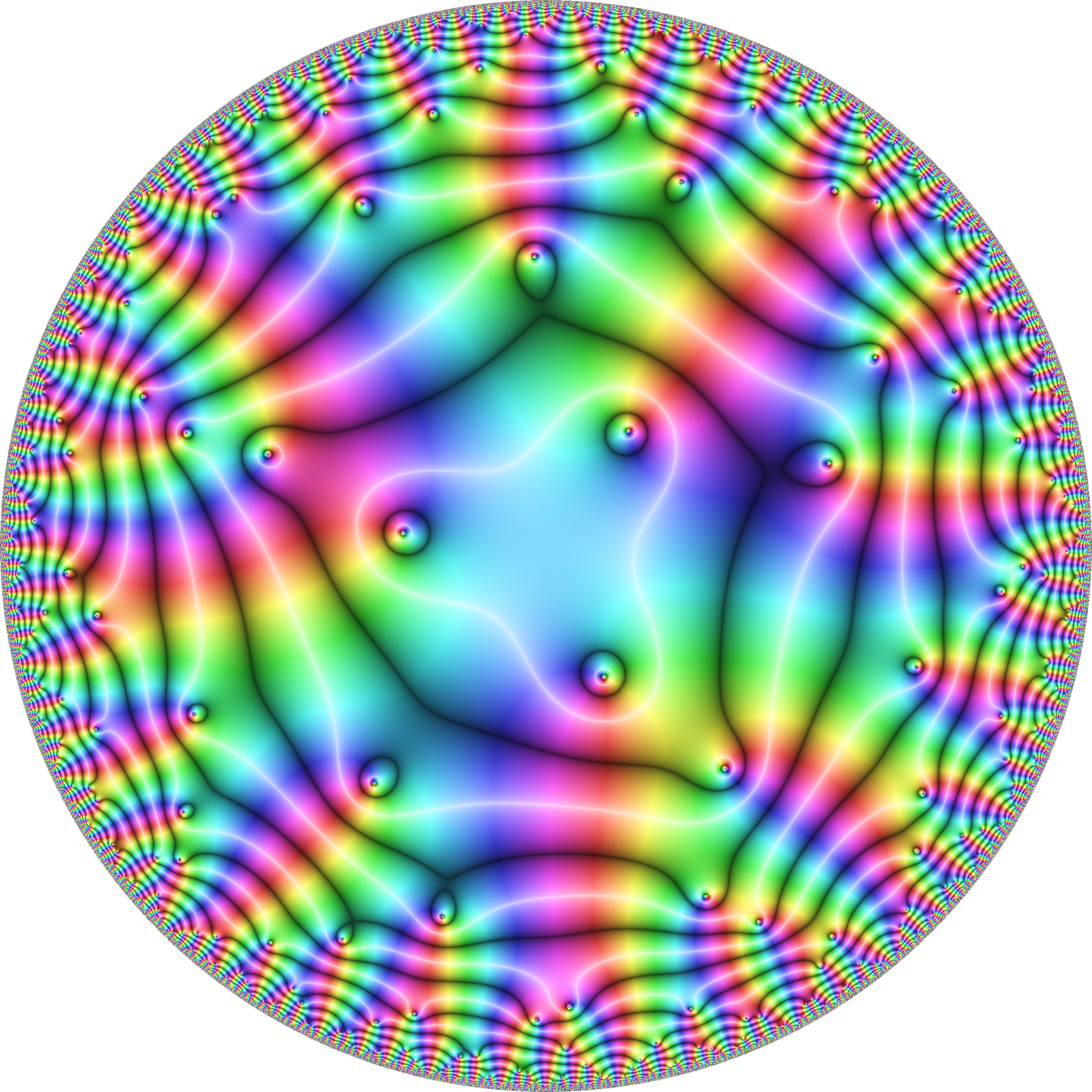
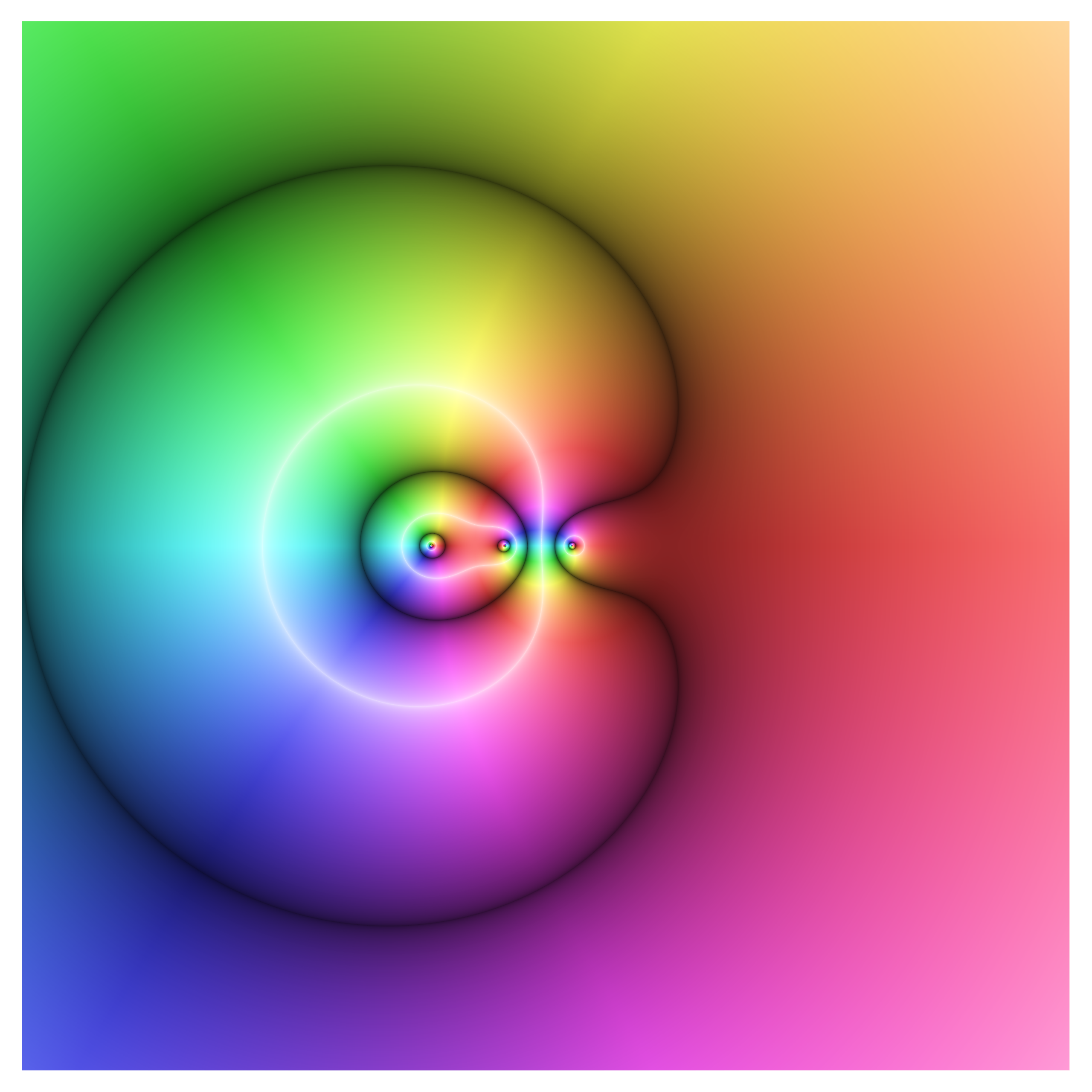
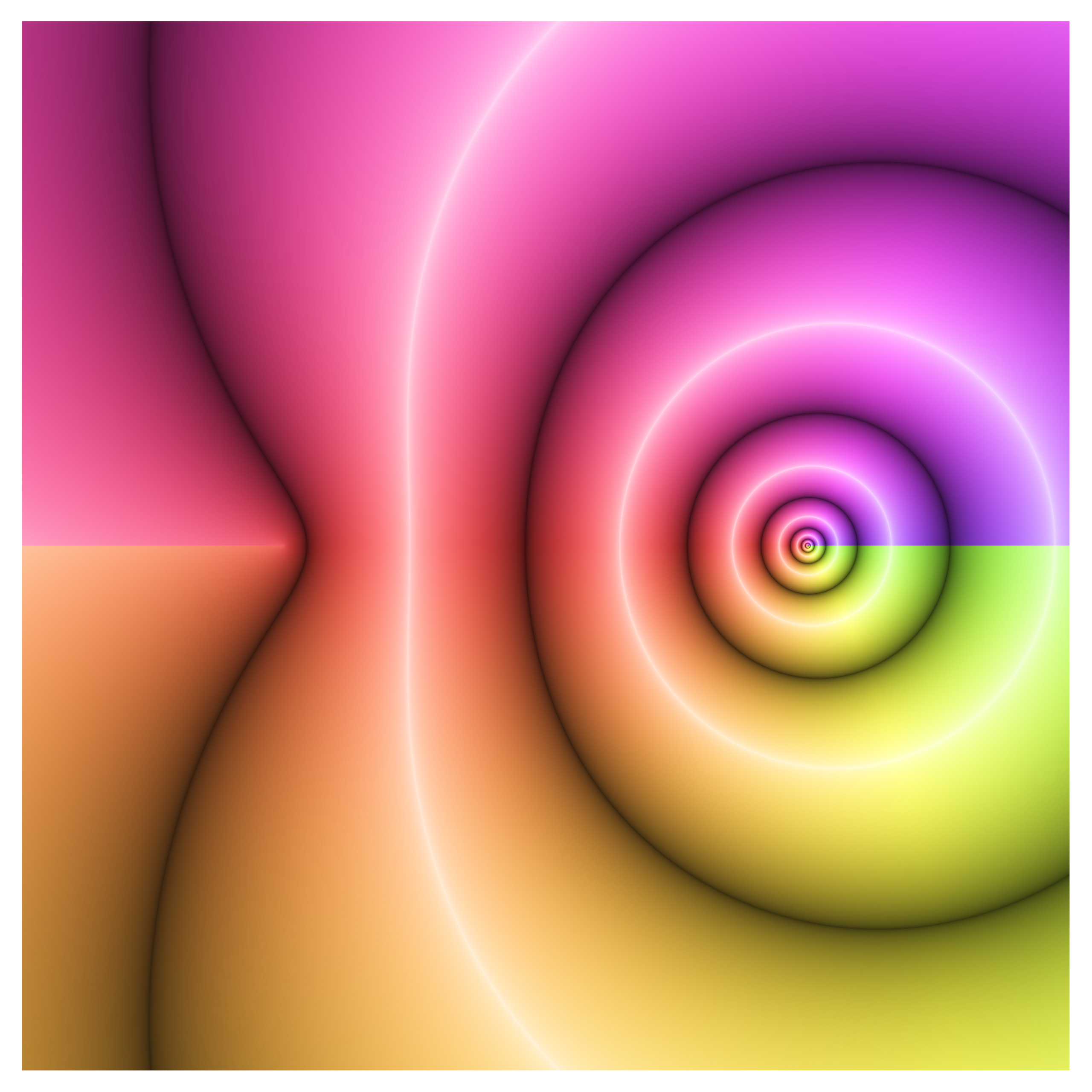
Derivatives of some random Fibonacci lacunary series.
The first image is a lacunary series with random coefficients, with only terms in the series whose powers are in the Fibonacci series. Since the Fibonacci series is lacunary, the disk must be a natural boundary, but it is not clear from the image why this is. Taking derivatives has the effect of pulling the boundary behavior inwards, and we can see clearly that the derivatives of the function exhibit huge clusters of zeros. The original image actually has zeros clustering on the boundary as well, they are just too close for them to be visible. The Fibonacci sequence was chosen because we can see rings of zeros which match up with the monomial terms in the series.