Finite Element Methods
We use the linear finite element method for solving the Poisson equation as an example to illustrate the main ingredients of finite element methods. We recommend to read
Contents
Variational formulation
The classic formulation of the Poisson equation reads as

where  and
and  . We assume
  is closed and
  open.
open.
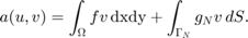
Denoted by  . Multiplying the Poisson equation by a test function
  and using integration by parts, we obtain the weak formulation of the Poisson equation: find
  such that for all
  :
:

Let  be a triangulation of
  . We define the linear finite element space on as

where  is the polynomial space with degree
  .
.
The finite element method for solving the Poisson equation is to find  such that for all
  :
:
Finite element space
We take linear finite element spaces as an example. For each vertex  of , let
  be the piecewise linear function such that
  and
and  when
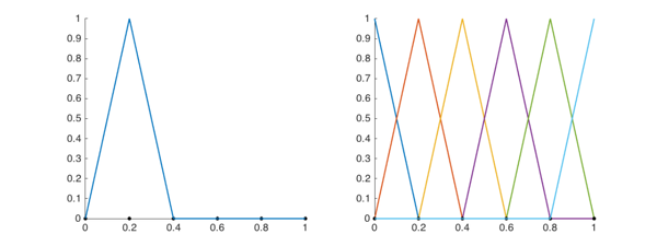
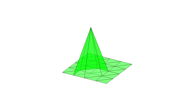
when  . The basis function in 1-D and 2-D is illustrated below. It is also called hat function named after the shape of its graph.
x = 0:1/5:1;
u = zeros(length(x),1);
u(2) = 1;
figure;
set(gcf,'Units','normal'); set(gcf,'Position',[0,0,0.5,0.3]);
subplot(1,2,1); hold on;
plot(x,0,'k.','MarkerSize',18);
plot(x,u,'-','linewidth',1.2);
subplot(1,2,2); hold on;
for k = 1:length(x)
    u = zeros(length(x),1); u(k) = 1;
    plot(x,0,'k.','MarkerSize',18);
    plot(x,u,'-','linewidth',1.2);
end
2-D hat basis
clf; set(gcf,'Units','normal'); set(gcf,'Position',[0,0,0.5,0.4]);
[node,elem] = squaremesh([0,1,0,1],0.25);
u = zeros(size(node,1),1);
u(12) = 1;
showmesh(node,elem,'facecolor','none'); hold on;
showsolution(node,elem,u,[30,26],'facecolor','g','facealpha',0.5,'edgecolor','k');
Then it is easy to see  is spanned by
  and thus for a finite element function
  .
.